Introduction to machine learning with tensorflow

If in the next five years we build a machine with the intellectual abilities of one person, then its successor will already be more intelligent than all humanity together. After one or two generations, they simply stop paying attention to us. Just as you do not pay attention to the ants in your yard. You do not destroy them, but you do not tame them, they have practically no effect on your daily life, but they are there.
Seth Shostak

Introduction

A series of my articles is an extended version of what I wanted to see when I decided to get acquainted with neural networks. It is designed primarily for programmers who want to get acquainted with tensorflow and neural networks. I do not know, fortunately or unfortunately, but this topic is so extensive that even a little bit informative description requires a large amount of text. Therefore, I decided to divide the narration into 4 parts:

1. Introduction, familiarity with tensorflow and basic algorithms (this article)
2. First neural networks
3. Convolutional neural networks
4. Recurrent Neural Networks

The first part set out below is aimed at explaining the basics of working with tensorflow and in passing telling how machine learning works in principle, using the example of tensorfolw. In the second part, we will finally begin to design and train neural networks, incl. multilayer and pay attention to some of the nuances of preparing training data and the choice of hyperparameters. Since convolutional networks are now very popular, the third part is dedicated to a detailed explanation of their work. Well, in the final part of the story about recurrent models is planned, in my opinion, this is the most difficult and interesting topic.

Tensorflow installation

Although the description of the installation of tensorflow is not the goal of the article, I will briefly describe the installation process of the cpu-version for 64-bit windows systems and add-ons used later in the text. In general, the installation procedure can be viewed on the website tensorflow.

1. Download and install python version 3.5. * (The latest version at the time of writing 3.5.3 ). During the installation, check the box “Add Python 3.5 to PATH”. If you do not want to add directories of this version of python to environment variables, for example, due to the active use of another version of the interpreter, then you should perform the further steps from the Scripts folder of the specified version of the distribution kit (cd "path to python 3.5 / Scripts").
   ')
   
2. After installation, run the command line (exactly after installation, otherwise the python directories will not get into the PATH environment variable).
   
   
3. Next, run the commands:
   
   
   1. pip update: "pip install --upgrade pip"
   2. setuptools update: "pip install -U pip setuptools"
   3. Installing tensorflow 1.0.1 under CPU: "pip install --ignore-installed --upgrade ci.tensor.org/view/Nightly/job/nightly-win/DEVICE=cpu , OS = windows / lastSuccessfulBuild / artifact / cmake_build / tf_python /dist/tensorflow-1.0.1-cp35-cp35m-win_amd64.whl »
   4. install matplotlib (for charts): “pip install matplotlib”
   5. Jupyter installation: "pip install jupyter"
      
4. The installation is complete, to launch Jupyter, execute the “jupyter notebook” command and in the opened tab you can open the ipynb version of the article ( take here ).

Below is a script for vbs , if you just want to quickly install all the necessary software, without going into details, then just run it and follow the instructions:

Introduction to tensorflow

The principles of working with tensorflow are quite simple. We must compile a graph of operations, then transfer data to this graph and give the command to make calculations. In the picture below you can see 3 examples of such graphs:

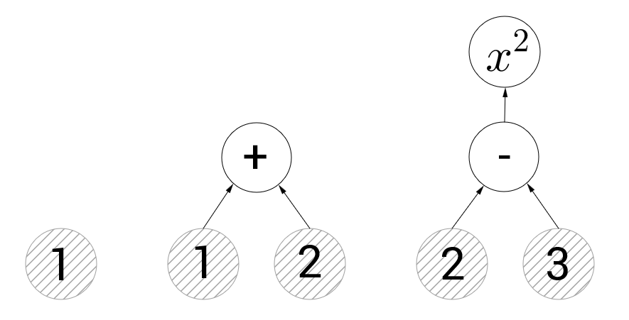
The graph on the left contains only one vertex representing a constant with a value of 1. Hereinafter, in such illustrations, vertices with constants will be indicated by circles with gray hatching, and without hatching vertices with operations. The central graph illustrates the addition operation. If we ask tensorflow to calculate the value of the vertex representing the operation of addition, it will calculate the values ​​of the edges of the graph directed to it and sum them (that is, it will return 3). In the right column we have two vertices with operations - subtraction and squaring. If we try to calculate the vertex representing the squaring, then the tensorflow will first perform the subtraction. I think the concept of computing graphs will not cause anyone any difficulties.

You can create an empty graph with the tf.Graph () function, besides, the graph is created by default when the library is connected and if you do not explicitly specify the graph, then it will be used. The example below shows how to create two constants in two different columns.

 import tensorflow as tf #       #   -   default_graph = tf.get_default_graph() #     - c1 = tf.constant(1.0) #    second_graph = tf.Graph() with second_graph.as_default(): #         c2 = tf.constant(101.0) print(c2.graph is second_graph, c1.graph is second_graph) # True, False print(c2.graph is default_graph, c1.graph is default_graph) # False, True 

Data transfer and operations take place in sessions. A session is started by calling tf.Session, and its closing by calling the close method on the session object. You can use the with clause, which automatically closes the session:

 default_graph = tf.get_default_graph() c1 = tf.constant(1.0) second_graph = tf.Graph() with second_graph.as_default(): c2 = tf.constant(101.0) session = tf.Session() #     - print(c1.eval(session=session)) # print(c2.eval(session=session)) #  ,    session.close() #  : with tf.Session() as session: print(c1.eval()) #       eval #   : with tf.Session(graph=second_graph) as session: print(c2.eval()) #       eval #: # 1.0 # 1.0 # 101.0 

I hope about the graphs and sessions in general, clearly, their functionality will not be understood in detail here, those who want to thoroughly understand these mechanisms should get acquainted directly with the documentation. And then we proceed to the construction of graphs. In the previous examples, constants were added to the graph, and it is time to find out what they are and how they differ from placeholders and variables. In the example below, a more complex graph is constructed representing the expression$$ $ inline $ a \ cdot x + b $ inline $ .

 #   a.           #       ,      : # a = tf.constant(2.0) #  : # value ( ) -   # shape - . : [] - , [5] -   5 , [2, 3] -  2x3(2   3 ) # dtype -   ,     https://www.tensorflow.org/api_docs/python/tf/DType # name -  .            a = tf.constant(2.0, shape=[], dtype=tf.float32, name="a") #   x #         #       ,    : # initial_value -     # dtype - , name - ,     x = tf.Variable(initial_value=3.0, dtype=tf.float32) #           ,      #       placeholder #          ,     #       b = tf.placeholder(tf.float32, shape=[]) #     ,        f = tf.add(tf.multiply(a, x), b) #     f = a*x + b with tf.Session() as session: #        #      x tf.global_variables_initializer().run() #     f   #   feed_dict    placeholder' #    b = -5 #      ,    result_f, result_a, result_x, result_b = session.run([f, a, x, b], feed_dict={b: -5}) print("f = %.1f * %.1f + %.1f = %.1f" % (result_a, result_x, result_b, result_f)) print("a = %.1f" % a.eval()) #   ,    #  eval    run  ,       ( feed_dict) #      ,   : x = x.assign_add(1.0) print("x = %.1f" % x.eval()) # : # f = 2.0 * 3.0 + -5.0 = 1.0 # a = 2.0 # x = 4.0 

So, a placeholder is a node through which new data will be transferred to the model, and a variable (Variable) is a node that may change as the graph runs. I hope that the above material is clear to everyone, because it is just enough to start learning the first model. In the previous code snippet we compiled a linear function graph$$ $ inline $ a \ cdot x + b $ inline $ , now let's go a little further and approximate the function$$ $ inline $ a \ cdot x + b $ inline $ over a set of points. Yes, I know that everyone has already been bothered by this task, as well as the recognition of characters and a series of cliche examples, but put up with it, you have to go through all of them ...

First learning algorithm

In order for tensorflow to train the model, we need to add 2 more things: the loss function and the optimization algorithm itself.

The loss function is a function that takes the value of the function predicted by the model and the actual value, and returns the distance between them (we will call this value an error). For example, if we predict a real value, then as the loss function, we can take the square of the difference of the arguments or the modulus of their difference. If we have a classification task, then the loss function can return 0 for the correct answer and 1 for errors. Roughly speaking, the loss function should return a non-negative real number and it should be the greater, the more the model makes a mistake, and then the task of training the model is reduced to minimization. And although the last sentence is not entirely correct, it fully reflects the idea of ​​machine learning.

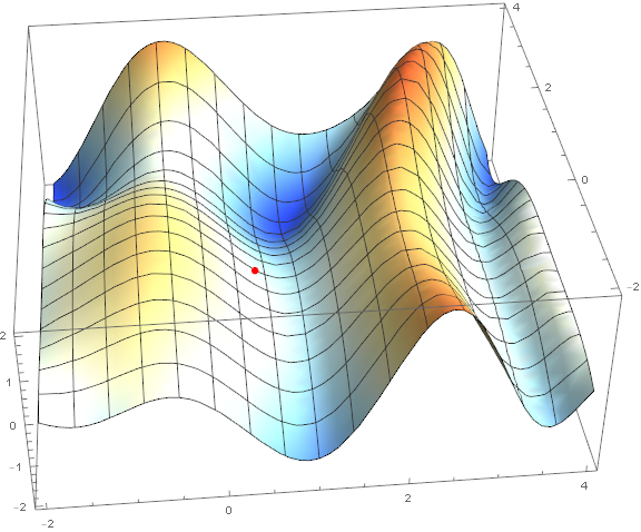
Of the optimization methods, we consider only the classical gradient descent. Much has already been written about him, so I will not disassemble it "brick by brick" and go into details (the material is not so small anyway). However, it must be understood, so I will try to explain the method briefly and clearly with the help of visualizations. Below are 2 options of the same schedule -$$ $ inline $ \ sin \ left (\ frac12x ^ 2- \ frac14y ^ 2 \ right) + \ cos (2x + 1) $ inline $ . The task of the method is to find a local minimum, i.e. from a point (taken at random, on a chart$$ $ inline $ \ left (\ frac12; \ frac12 \ right) $ inline $ ) get into the recess (blue zone in the graphs).


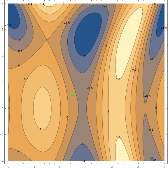
The essence of the method is to go in the direction opposite to the gradient function at the current point. The gradient is a vector that points in the direction of the largest growth of the function. Mathematically, this is a vector of derivatives for all arguments -$$ $ inline $ \ mathrm {grad} (f) = \ nabla f = \ left (\ frac {\ partial f} {\ partial x}, \; \ frac {\ partial f} {\ partial y} \ right) $ inline $ . The function is taken at random and we will not carry out calculations on it, for practice we have a simpler example, first look at the visualization of several steps of the algorithm:


Separately, it is worth mentioning the speed with which you need to move to a minimum (with reference to the machine learning task, this will be called the learning rate). To get the first results, we just need to pick a fixed speed. However, it is often a good idea to lower it in the course of the algorithm, i.e. move less and less steps. While this is sufficient, we will analyze the method in more detail with practice, as necessary.

In the following example, we will try to restore the value of the function$$ $ inline $ 2x-3 $ inline $ on the interval from -2 to 2 by 50 points with normally distributed noise. We will train the model in sets (packages) of 5 points each using a stochastic gradient descent (eng. SGD - Stochastic Gradient Descent). Let's go straight to the code.

 import numpy as np import tensorflow as tf %matplotlib inline import matplotlib.pyplot as plt samples = 50 #   packetSize = 5 #   def f(x): return 2*x-3 #   x_0 = -2 #   x_l = 2 #   sigma = 0.5 #    np.random.seed(0) #    (          ) data_x = np.arange(x_0,x_l,(x_l-x_0)/samples) #  [-2, -1.92, -1.84, ..., 1.92, 2] np.random.shuffle(data_x) # ,    data_y = list(map(f, data_x)) + np.random.normal(0, sigma, samples) #      print(",".join(list(map(str,data_x[:packetSize])))) #    print(",".join(list(map(str,data_y[:packetSize])))) #     tf_data_x = tf.placeholder(tf.float32, shape=(packetSize,)) #        tf_data_y = tf.placeholder(tf.float32, shape=(packetSize,)) #        weight = tf.Variable(initial_value=0.1, dtype=tf.float32, name="a") bias = tf.Variable(initial_value=0.0, dtype=tf.float32, name="b") model = tf.add(tf.multiply(tf_data_x, weight), bias) loss = tf.reduce_mean(tf.square(model-tf_data_y)) #  ,    optimizer = tf.train.GradientDescentOptimizer(0.5).minimize(loss) #  ,     with tf.Session() as session: tf.global_variables_initializer().run() for i in range(samples//packetSize): feed_dict={tf_data_x: data_x[i*packetSize:(i+1)*packetSize], tf_data_y: data_y[i*packetSize:(i+1)*packetSize]} _, l = session.run([optimizer, loss], feed_dict=feed_dict) #     "" print(": %f" % (l, )) print("a = %f, b = %f" % (weight.eval(), bias.eval())) plt.plot(data_x, list(map(lambda x: weight.eval()*x+bias.eval(), data_x)), data_x, data_y, 'ro')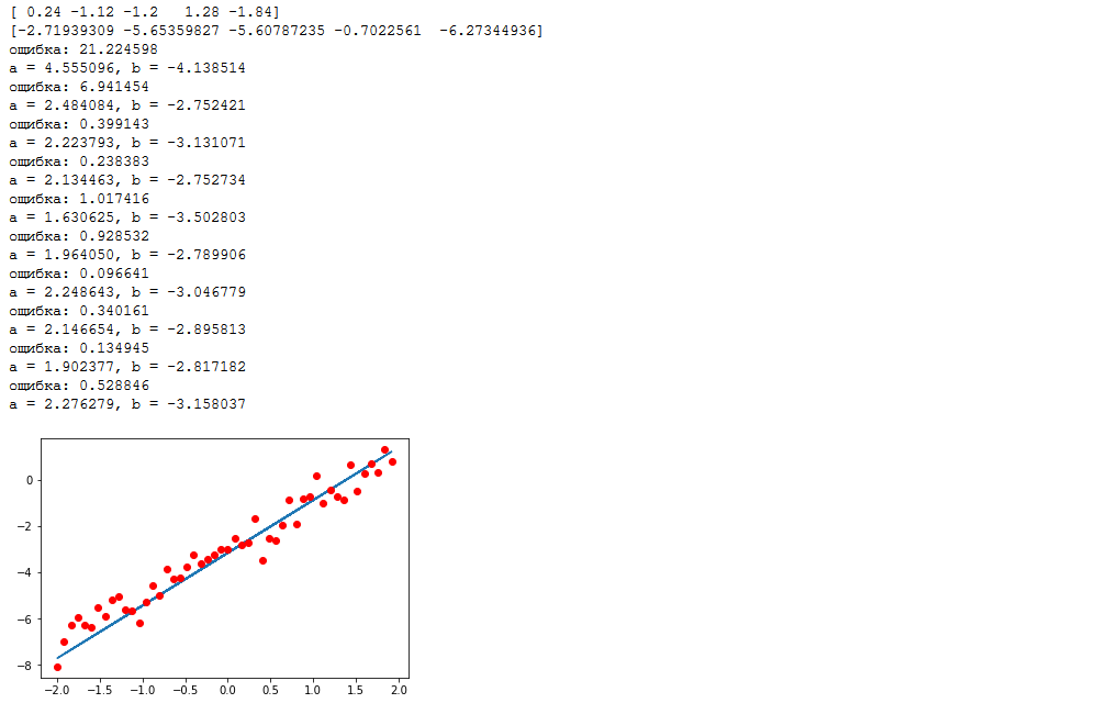 

Our graph looks like this:

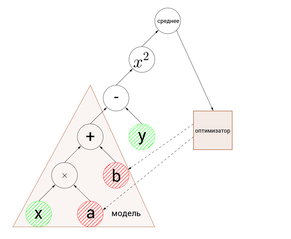
input nodes are highlighted in green, and variables to be optimized in red.

The first thing that should be noticed is the discrepancy between the dimensions of the input nodes and the variables. Input nodes accept arrays of 5 elements each, and variables are numbers. This is called batch computing (broadcasting) . Roughly speaking, when it is necessary to perform calculations on arrays, one of which has an extra dimension, calculations are performed separately for each element of a larger array and the result will be an array of greater dimension. Those. [1,2,3,4,5] + 1 = [2,3,4,5,6], it is rather difficult to formulate, but it should be intuitively clear.

Let's manually recalculate the actions of the algorithm, I think this is the best way to understand what is happening. So, the arguments are passed to the inputs - [0.24, -1.12, -1.2, 1.28, -1.84] and the values ​​[-2.72, -5.65, -5.61, -0.70, -6.27] (rounded to hundredths). First, we batchly calculate the value of the function, let me remind you that after initializing the variables, the function looks like$$ $ inline $ 0.1 \ cdot x + 0 $ inline $ . We substitute each argument:

$$$$ display $$ \ left [\ begin {matrix} 0.1 \ cdot 0.24 + 0 = 0.024 \\ 0.1 \ cdot -1.12 + 0 = -0.112 \\ 0.1 \ cdot -1.2 + 0 = -0.12 \\ 0.1 \ cdot 1.28 + 0 = 0.128 \\ 0.1 \ cdot -1.84 + 0 = -0.184 \ end {matrix} \ right. $$ display $$

Further, the obtained values ​​are subtracted from the reference values, squared and the average value is calculated:

$$$$ display $$ \ left [\ begin {matrix} (0.024 - (- 2.72)) ^ 2 \ approx7.53 \\ (-0.112 - (- 5.65)) ^ 2 \ approx30.67 \\ (- 0.12- (-5.61)) ^ 2 \ approx30.14 \\ (0.128-0.7) ^ 2 \ approx0.69 \\ (- 0.184 - (- 6.27)) ^ 2 \ approx37.04 \ end {matrix} \ right. \ Rightarrow \ frac {7.53 + 30.67 + 30.14 + 0.69 + 37.04} 5 \ approx21.21 $$ display $$

a difference of about one hundredth from the value displayed in the log is caused by rounding to hundredths during calculations. So, we considered a mistake, now it's time to figure out the optimization. In the graph above, dotted arrows indicate that the optimizer changes variables. You should already have an intuitive understanding of how gradient descent works. In this example, a stochastic gradient descent with a speed of 0.5 is used. Let's take it in order, we optimize the variables a and b, so by them we find the gradient:

$$$$ display $$ f = (a \ cdot x + b - y) ^ 2 \ Rightarrow \ left \ {\ begin {matrix} \ frac {\ partial f} {\ partial a} = 2x (ax + by) \ \\ frac {\ partial f} {\ partial b} = 2 (ax + by) \ end {matrix} \ right. $$ display $$

We need to improve the value over the entire set of points, so we calculate the average value of the gradient, for convenience, for each variable separately:

$$$$ display $$ \ begin {matrix} a \ Rightarrow \ frac {1.31712 + (- 12.4051) + (- 13.176) +2.11968 + (- 22.3965)} {5} = - 8.90816 \\ b \ Rightarrow \ frac {5.488 + 11.076 + 10.98 + 1.656 + 12.172} {5} = 8.2744 \ end {matrix} $$ display $$

And finally, we change the values ​​of the variables to be optimized, taking into account the given speed:

$$$$ display $$ \ begin {matrix} a_ {new} = a_ {old} -0.5 \ cdot-8.90816 = 0.1-0.5 \ cdot (-8.90816) = 4.55 \\ b_ {new} = b_ {old} -0.5 \ cdot8.2744 = 0-0.5 \ cdot (-8.90816) = - 4.14 \ end {matrix} $$ display $$

Meanings$$ $ inline $ a_ {new} $ inline $ and$$ $ inline $ b_ {new} $ inline $ and there are the desired values ​​of variables. These calculations are repeated in a loop on each set of points. Why is this method called stochastic? Because we calculate the gradient only on a small piece of data (package), and not on all points at once. Thus, stochastic descent requires much less computation, but does not guarantee a reduction in error at each iteration. Oddly enough, this “noise” in terms of the convergence in time can even be useful, since allows to "get out" from local minima.

Actually, this is still possible to finish. The article turned out even relatively small, which is good. I am writing this kind of material for the first time, so if you think that the article doesn’t discuss some of the points in sufficient detail or in the wrong way, please write about it - the article will definitely be updated and corrected based on constructive criticism. In addition, it will help to better prepare for publication subsequent parts, which will necessarily be posted here (of course, except for the scenario in which the article will be met negatively).

In conclusion, I would very much like to thank my friend Nikolai Saganeniko for help in preparing the material. It is thanks to him that my small cheat sheet for personal use turned into the foregoing stream of consciousness.