M * - the shortest path search algorithm, through the whole world, on a smartphone

When searching for the shortest path on large graphs, the traditional cost estimate does not work well because the data is obviously not fit in memory and the total cost depends more on the number of disk accesses than on the number of edges scanned. And the number of disk operations is a very subjective factor, depending on the difficultly formalizable suitability of a graph for disk storage in the form convenient for a specific algorithm. In addition, compactness becomes very important - the amount of information per edge and vertex.

Under the cat, there is a generalized heuristic to the algorithm A *, which is useful precisely in the light of practical suitability on large graphs with limited resources, for example, on a mobile phone.

So, our task is to build the shortest path along a graph from point to point. At the same time, the graph is large enough so that we would not be able to keep it entirely in memory, and it is also impossible to pre-calculate for any significant number of vertices. A great example is the OSM road graph. Currently, the number of vertices in OSM has exceeded 4.6 billion, the total number of objects is 400 million.
')
It is clear that in such conditions, the search for a more or less extended route with a pure Dijkstra or Levitic algorithm is impossible due to the fact that we do not have the amount of memory required to store intermediate data.

What is the Dijkstra algorithm doing?

1. Bring in a priority queue starting point with zero cost.
2. While there is something in the queue - let the vertex V, for each outgoing edge (E), which we have not yet viewed:
   
   1. check that this is not the desired edge, if so, then the end;
   2. calculate the cost of passage E;
   3. and put the final vertex of the edge E in the queue with the cost of its achievement - the cost of achieving V + cost E.

As a result, for sparse (for example, geometric) graphs, we obtain the value O (n * log (n) + m * log (n)), where n is the number of viewed vertices, m is the number of viewed edges.



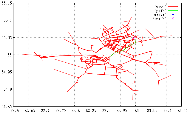
Figure 1 Here we see the route found and the edges scanned.

The problem is that Dijkstra's algorithm does not use any information about the properties of the graph and the desired route, and during its operation (propagation of the so-called “wave”), the perimeter of this “wave” moves from the desired point in all directions without any discrimination.

On the other hand, on geometric graphs, for example, a developed road network, it makes sense to stimulate the propagation of the “wave” towards the target and penalize for other directions. This idea is implemented in the A * algorithm, which is a generalization of the Dijkstra algorithm.

In A *, the cost of the vertex when it is placed on the priority queue is not just equal to the distance traveled, but also includes an assessment of the remaining path. How do we get this estimate?

It should be noted that this should be a fairly computationally cheap estimate since it is executed a large number of times. The first thing that comes to mind is to calculate the geometric distance from the current point to the finish line and proceed from this, for example: 10 km left - the average speed when driving through the city is 20 km / h, which means our estimate is half an hour.

In this case, if the edge leads us towards the finish line, the score for it will decrease and compensate for the distance traveled.

For the edges leading from the target, this estimate will increase, as a result such points will fall into a queue with a lot of weight and it is quite likely that the matter will not reach them.

Approximately the same effect can be achieved, by the way, using the Beam Search technique, where the size of the priority queue is forcibly limited and candidates that are “unworthy” from a heuristic point of view are simply discarded.



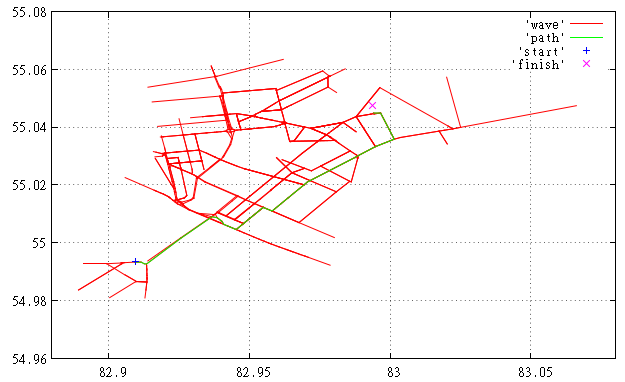
Figure 2 Here we see the search for the same route using the described heuristics, feel the difference.

A * turns into Dijkstra's algorithm if the cost estimate returns 0, as if we thought that the rest of the path would rush at infinite speed.

A * refers to the so-called. informed algorithms in heuristics, we use the assumption that moving towards a goal will rather lead us to success.

What should be the properties of the evaluation function? It should be believable. As we have already found out, too optimistic evaluation negates our attempts to reduce the visible part of the graph. On the other hand, a too pessimistic assessment will force the algorithm to build a path strictly along the direction, no matter what. It is unlikely that we are satisfied.

A realistic estimate should be based on the properties of the graph and better on the data model. For example, calculated from the level of congestion at this time of day and the level of transport connectivity of the graph. For example, in a city without rivers, the Manhattan distance works well.

But then immediately there is a mass of nuances:

• How to determine that we are in the city? It is not so cheap.
• And nothing that most of the cities built on the rivers?
• In the city, different sections of roads can be loaded heavily in different ways.
• And if we have to drive through many cities and rivers?

You can use different heuristics in the spirit of the branch and bound method :

1. We find a way with a very pessimistic heuristics, which means that, presumably, there are more efficient routes.
2. Now we will use the cost of the found route as an estimate from above, simply by not including in the priority list applicants who obviously cannot give us a route more efficient than the one already found.
3. We make the assessment less pessimistic and re-build the route with the upper limit of cost.
4. We get a new assessment.
5. We continue this way until we get a satisfactory solution.

There is another problem with the valuation, which is worth mentioning.

In life, geometrically close objects can be quite remote from the point of view of the road graph. For example, being on different sides of a river, a mountain range, the sea ... In this case, an assessment based on geometric proximity will begin to aggravate the situation, stubbornly directing the "wave" in the wrong direction.



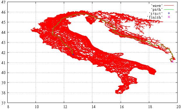
Figure 3 This is what the viewed A * part of the OSM graph looks like for finding a route from Italy to Albania.

However, it is still better than the algorithm Dijkstra. You can clearly see how filling the whole of Italy, the "wave" began to overflow, picked up speed and quickly reached the goal.



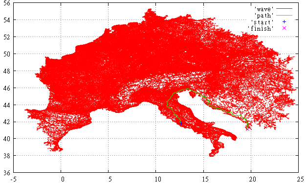
Figure 4 And this is how the scanned part of the graph looks for the Dijkstra algorithm. Compared to her, everything is not so gloomy.

Is it possible to somehow improve the algorithm, what does Computer Sience say about this?

Bidirectional search

You can send two A * waves towards each other. This is called bidirectional search and at first glance seems like a very attractive idea. In fact, with good transport connectivity, the “wave” is an ellipsoid, two small waves, directed towards, will notice a smaller area compared to one large. On the other hand, the problem of detecting a meeting of "waves" arises, there can be quite a lot of points in their perimeters and checking at every step the presence of an edge in someone else's perimeter is not so cheap.



Figure 5 oncoming Dijkstra waves

Perhaps this could be reconciled with a real gain in the volume of the scanned part of the graph. But if we consider the above example of finding a passage from Italy to Albania, we will find that bidirectional search will not help us, but will only aggravate the situation. in addition to pouring the whole of Italy, we will have to look through all of Greece and a half of the Balkans before the waves meet. For instead of one “wave”, resting on an obstacle, we will have two such.

Hierarchical approaches

Using road hierarchies

Some commercial systems, such as StreetMap USA , use for routing the fact that a well-planned road network has a two-tier nature - there is a network of local roads and a (much smaller) highway network for long-distance travel. It seems natural to use this fact. Introduced gateways (transit nodes) - the vertices at which the transition from one level to another. Finding a “long enough” path comes down to finding paths from:

• starting point to several nearby gateways;
• several nearest gateways to the final point;
• The shortest route from any of the initial gateways to any of the final ones, of course, is done in one session.

6 Slice StreetMap

The benefits of this approach are obvious. The downsides are:

• Not everywhere the road network is well planned, in some places it has grown spontaneously, therefore, the initial message does not work.
• Upper-level network must be connected and verified. From OSM, for example, it is impossible to get such a network (with a slight movement of the hand) simply by filtering the roads by classes.
• The gateway institute also requires a lot of manual work.

Construction of the graph hierarchy

If there is no possibility and / or desire to verify the graph, it remains possible to build a hierarchy automatically.

One way or another, the idea is being exploited that even though the graph is not verified, nevertheless, the attributes of the ribs allow us to build routes of acceptable quality. But due to the size of the graph, the construction of the same A * in the operating mode is prohibitively expensive.

For example, it might look like this:

• at the stage of pre-calculation, a set of (even random) vertices is selected;
• for pairs of spatially distant vertices, the usual A * shortest routes are constructed;
• on the basis of the constructed routes statistics of the passed edges is kept;
• after a sufficient amount of data has been accumulated, the visited edges are declared as the next level of the hierarchy;
• consecutively reaching edges without branches merge into a “macro pattern” while maintaining the cost of travel;

The constructed graph can again be subjected to the described procedure, thus building the required number of hierarchies.

Routing in such a hierarchical graph is performed by bidirectional search (A * or Dijkstra's algorithm).

Separators

The main idea of ​​the method is an attempt to divide the graph into components by removing a small part of the edges - separators. These separators and the pre-computed paths between them form the next hierarchy. It is stated [1] that by spending O (n * log (n) ** 3) time and disk space for preliminary calculation, you can execute queries in O (sqrt (n) * log (n))

Grid based transit nodes

This is generally the same idea with separators, but for purposes of scaling and simplicity, the graph is divided into fragments by a lattice or quadro-tree, the edges that cross the boundaries of the fragments become transit. It is clear that the price of this - efficiency. In the pros - high automation and, as a consequence, the absence of the human factor.

Distance tables

At the higher levels of the hierarchy in the process of searching for the path are not searched, and the cost is calculated on the basis of pre-calculated tables of the distances between the transit nodes. When the route is defined, the paths are restored by a local search.



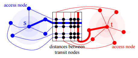
7 [1]

Reach [3]

The idea of ​​the method is as follows - it is noted that when building long optimal routes, “local” edges are visited only at the very beginning or end of the route. Consequently, having built a certain number of “training” long routes, one can understand how close one or another edge is to any of the ends of the route.

For some training route P (s ... ..uv ... ... t), the indicator reach is entered - the minimum distance to the ends reach (uv) = min (dist (s ... ..u), dist (v ... ..t)) .
On the entire training set, reach (uv) is the maximum value on all routes where the edge (uv) is encountered.

When “fighting” the search, we are far from the start and finish just going to try to avoid edges with a small value of reach.



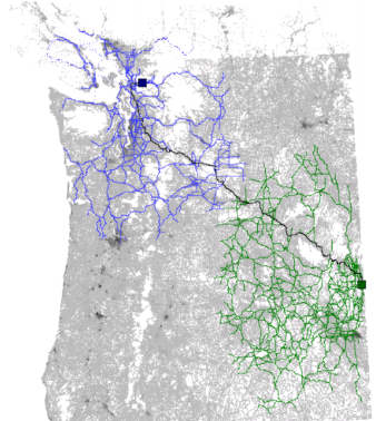
Fig.8 [21]

The idea of ​​the method is very beautiful, the questions are only the quality of the training sample, its sufficiency and resources spent on training.

Purposeful algorithms

Arc-Flags [4]

The graph is divided into fragments. Training on building the shortest route between predefined points. When constructing a training path, for each edge the fact that the shortest route to the final point cell passes through it is preserved.

Thus, for each edge we keep a flag mask, which fragments of the graph can be reached through this edge by the shortest path.

The specific disadvantages of this method are visible to the naked eye:

• The number of graph fragments can not be large, 8K fragments (which is not so much) will give us a (presumably incompressible) kilobyte per edge. Sic!
• You have to be very careful with slicing fragments; inside the fragment, the graph must be connected.

ALT [5]

A small number of landmarks is selected from all the vertices: λ. In the initial version, for each vertex, the values ​​were pre-calculated up to each λ. This required a tremendous amount of additional memory and in the future the requirements were softened and the peaks began to be grouped.

ALT searches are performed as in A *, but the remaining path is estimated based on the calculated values. Let we consider the edge (u, v) on the way to the target vertex t. For each λ, in accordance with the triangle inequality, we have an estimate of the remaining part of the path (via λ): dist (λ, t) - dist (λ, v) ≤ dist (v, t) and dist (v, λ) - dist (t , λ) ≤ dist (v, t). The minimum for all λ and give the desired estimate.



9

Preliminary results

We see two main areas in which development is underway:

1. Hierarchy. They allow you to very effectively build paths at large distances in structured graphs. But at short distances it is cheaper to use the usual A * or Dijkstra. Therefore, there is a “gray” area where both algorithms work mediocre.
   
   In addition, an attempt to build a hierarchy on amorphous graphs can only lead to problems. Imagine a graph in the form of a rectangular lattice of equivalent roads. When moving in a certain direction, the correct decision will turn in a random direction with a probability associated with the direction. Those. if the azimuth to the target is 45 °, you should turn right and left with equal probability, so as not to create traffic jams.
   
   An attempt to build a hierarchy on such a grid will result in inefficient use of the road network.
   
   
2. Using the internal nature of the graph to decide on the direction of movement to the goal. The idea looks promising, but it raises many questions. The main problem is the human factor. What lanmark'i, that fragments of Arc-Flags require the participation of an expert, if you let their definition of gravity, it is easy to get not what the doctor ordered.
   
   In addition, the amount of additional memory (non-linear from the graph size) is required.
   

Here, “if Nikanor Ivanovich’s lips were to be attached to Ivan Kuzmich’s nose, but to take some kind of swagger, like Balthazar Baltazarovich’s, yes, perhaps ...” ©

It is fair to say that there are many such attempts, some of them can be found in the list of sources of this article. But we, of course, will not change ourselves and come up with our own, “unparalleled” method. ️

Heuristic

We set the task to develop a simple and cheap (both computationally and from the point of view of additionally stored information) heuristics for estimating the cost of a path from one point to another based on their geographical coordinates. Direct distance does not fit, it can be very wrong, just look at Gibraltar and Tangier.

The idea goes back to this work.

• Since we are working with OSM, the scale of the graph is the whole planet.
• We divide the space with a grid of 1 °, yes, it gives distortions to the poles, but we are developing only an estimate.
• When constructing the graph, we will rasterize the paths on this grid, for example, for the 2nd Krupskaya lane in Novosibirsk, we must mark the checkbox corresponding to 55 ° N. and 82 ° E
• After rasterization of all roads known to us, we get a population map with an accuracy of a degree.
  
  
  
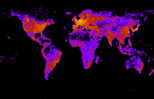
  Figure 10 - the number of roads per square degree on a logarithmic scale.
  
  
• We will consider our map as a graph, where populated cells are vertices.
• We assume that if neighboring cells are inhabited, then this is an edge, from one can be passed to another, the cost of direct travel is 111 km at the equator, the fare is diagonally multiplied by the root of 2.
• If in this graph we launch a wave in accordance with the Dijkstra algorithm, remembering the cost of reaching each vertex, it will give us an estimate of the cost of the way to the finish at any achievable point. For example, if you let a wave out of Novosibirsk, it will look like this:
  
  
  
  11 Estimate the cost of travel from Nsk, the closer to orange, the longer the path.
  

So, for the search:

• We store only bits per square degree of surface.
• Once we start a wave on this bitmap for the final point.
• For any vertex in the graph, knowing its coordinates, for a constant time we get an estimate of the cost of travel from this point to the finish.

But the degree is a rather coarse grid, some straits may stick together, for example, a “small island” with Normandy.

It does not matter, in OSM there is a type - a coastline. We will rasterize coastlines and allow walking from a cell labeled coastal to the “mainland” cells.


Fig Coastline OSM

But it turns out that:

• the coastline is not everywhere;
• Japan et al. Consists entirely of coastal cells;
• Gibraltar and Tangier are in the same cell;
• ...

Ok, you have to draw the dividing lines in important straits with your hands, rasterize them and prohibit them to cross when the wave propagates.

Fortunately, this is a one-time job, and there are not very many such straits.

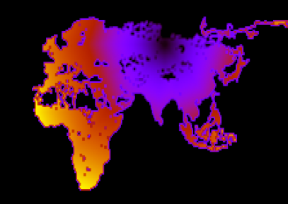
For example, the spread of "waves" from Italy, pay attention to the Strait of Gibraltar.



Fig.13 Estimated cost of travel to Italy, the closer to orange, the longer the path.

In general, the scheme is acceptable, but:

1. it requires manual work;
2. a lot of handmade;
3. one must be very careful if several dividing lines lay on one cell.

It is possible that the variant when each “coastal” cell is represented by a quad-tree will work well here, and wave propagation should be carried out along the elements of the quadtree.

But still there is a stretch in all this, so Plan B. enters the business.

Plan b.

1. Suppose we have a higher level hierarchy of the graph, obtained, for example, by the method described in the section “Construction of the graph hierarchy”.
2. This level is rude enough so that searching for any distance in it does not pose a problem.
3. So, we have in our hands a path built on a higher level of the graph hierarchy.
   
   
   
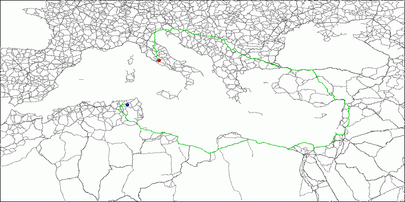
   Fig.14 The path laid on the top-level graph.
   
   
4. We will put reference points on this route, for example, every 500 km, including the finish, of course
   
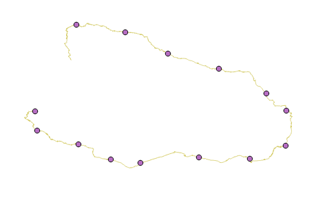
   Fig Reference points.
   
5. For each pivot point we know the rest of the way from it to the finish. Now the remainder heuristics for A * will consist of two parts:
   
   1. geometric distance to the current reference point;
   2. the rest of the way from the current reference point to the finish.
6. At the beginning of the search, the current reference point is assigned. As soon as we approach it at a geometric distance closer than 200 km (conventionally, of course), we begin to focus on the next reference point. And so to the finish.
7. The result is:
   
   
   
   FIG. 11 It is clearly seen how the wave begins to spread outward when the reference path changes its direction abruptly. However, the total amount of read data is very small. There is also an acceleration of ~ 20 times.
   
   
8. Most of all, this technique resembles the image from the cap for this article. Therefore, the author gave her the name M * (“M” means “carrot”).

findings

So, the reader is presented with two options for the heuristics of calculating the cost of the remainder of the path for A *.

For both options:

• tested their performance in practice;
• the speed of work A * is about the same, for the specified path it is 4.5 seconds (an ordinary desktop) with reading and unpacking data, 0.5 seconds - only the passage of a wave on a heated cache;
• the amount of additionally stored information is minimal - 0.2% for the second option, for the first even less;
• because A * works with the original graph, there are no obstacles to the use of time constraints, for example, ferries, movable bridges, traffic data ...

Be that as it may, this is another tool for working with graphs, very useful in conditions of limited resources and / or unlimited data. In particular, no one forbids using the same technique for a two-way search.


PS : article on the results of the report on the DUMP 2017