Open machine learning course. Topic 8. Gigabyte training with Vowpal Wabbit

Hello!

Here we are gradually and have come to advanced methods of machine learning. Today we will discuss how to approach the training model in general, if the data is gigabytes or tens of gigabytes. Let's discuss the techniques that allow doing this: stochastic gradient descent (SGD) and feature hashing, let's look at examples of using the Vowpal Wabbit library.

UPD: now the course is in English under the brand mlcourse.ai with articles on Medium, and materials on Kaggle ( Dataset ) and on GitHub .

Video recording of the lecture based on this article as part of the second launch of the open course (September-November 2017).

List of articles series

Plan

Stochastic Gradient Descent and Online Learning Approach

Stochastic Gradient Descent

Despite the fact that gradient descent is one of the first topics studied in optimization theory and machine learning, it is difficult to overestimate the importance of one of its modifications - the stochastic gradient descent, which we will often call simply SGD (Stochastic Gradient Descent).

Recall that the essence of the gradient descent is to minimize the function, taking small steps towards the steepest decrease of the function. The name of the method was presented by the fact from the mathematical analysis that the vector $\ nabla f = (\ frac {\ partial f} {\ partial x_1}, \ ldots \ frac {\ partial f} {\ partial x_n}) ^ T$ partial derivatives of a function $f (x) = f (x_1, \ ldots x_n)$ sets the direction of the fastest increase of this function. So, moving in the direction of the anti-gradient function, you can reduce the values of this function the fastest.

This is me in Sheregesh - I advise everyone who rolls to be there at least once in their life. Picture to soothe the eyes, but with its help you can explain the intuition of the gradient descent. If the task is to go down the mountain on a snowboard as quickly as possible, then you need to choose the maximum slope at each point (if it is compatible with life), that is, calculate the antigradient.

Example: steam regression

The problem of simple pair regression can be solved using a gradient descent. Suppose we predict one variable for another — growth in weight — and postulate a linear dependence of height on weight.

Code reading data and drawing a scatterplot

%matplotlib inline from matplotlib import pyplot as plt import seaborn as sns import pandas as pd data_demo = pd.read_csv('../../data/weights_heights.csv')

 plt.scatter(data_demo['Weight'], data_demo['Height']); plt.xlabel('  ') plt.ylabel('  ');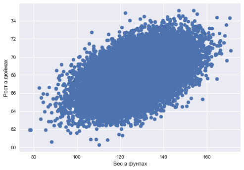

Dana vector $x$ lengths $\ ell$ - weight values for each observation (person) and $y$ - vector of growth values for each observation (person).

Task: to find such weights $w_0$ and $w_1$ so that when the prediction of growth in weight in the form $y_i = w_0 + w_1 x_i$ (Where $y_i$ - $i$ -th growth value, $x_i$ - $i$ -th weight value) to minimize the quadratic error (it is possible and the root mean square, but constant $\ frac {1} {\ ell}$ the weather does not, and $\ frac {1} {2}$ instituted for beauty):

S E (w_{0}, w_{1}) = f r a c 12 s u m_{i = 1}^{} e l l (y_{i} - (w_{0} + w_{1} x_{i}))^{2} r i g h t a r r o w m i n_{w_{0}, w_{1}}

$SE (w_0, w_1) = \ frac {1} {2} \ sum_ {i = 1} ^ \ ell (y_i - (w_0 + w_1x_ {i})) ^ 2 \ rightarrow min_ {w_0, w_1}$

We will do this using a gradient descent, counting the partial derivatives of the function $SE (w_0, w_1)$ by weights in the model - $w_0$ and $w_1$ . The iterative learning procedure will be defined by simple weights update formulas (we change the weights so as to make a small, proportionally small $\ eta$ , step towards the anti-gradient function):

b e g i n a r r a y r c l w_{0}^{(t + 1)} = w_{0}^{(t)} - ​ ​ e t a f r a c p a r t i a l S E p a r t i a l w_{0} |_{t} w_{1}^{(t + 1)} = w_{1}^{(t)} - ​ ​ e t a f r a c p a r t i a l S E p a r t i a l w_{1} |_{t} e n d a r r a y

$\ begin {array} {rcl} w_0 ^ {(t + 1)} = w_0 ^ {(t)} - \ eta \ frac {\ partial SE} {\ partial w_0} | _ {t} \\ w_1 ^ {(t + 1)} = w_1 ^ {(t)} - \ eta \ frac {\ partial SE} {\ partial w_1} | _ {t} \ end {array}$

If we turn to the pen and paper and find analytical expressions for partial derivatives, we get

b e g i n a r r a y r c l w_{0}^{(t + 1)} = w_{0}^{(t)} + e t a s u m_{i = 1}^{e l l} (y_{i} - w_{0}^{(t)} - w_{1}^{(t)} x_{i}) w_{1}^{(t + 1)} = w_{1}^{(t)} + e t a s u m_{i = 1}^{e l l} (y_{i} - w_{0}^{(t)} - ​ ​ w_{1}^{(t)} x_{i}) x_{i} e n d a r r a y

$\ begin {array} {rcl} w_0 ^ {(t + 1)} = w_0 ^ {(t)} + \ eta \ sum_ {i = 1} ^ {\ ell} (y_i - w_0 ^ {(t) } - w_1 ^ {(t)} x_i) \\ w_1 ^ {(t + 1)} = w_1 ^ {(t)} + \ eta \ sum_ {i = 1} ^ {\ ell} (y_i - w_0 ^ {(t)} - w_1 ^ {(t)} x_i) x_i \ end {array}$

And all this works quite well (in this article we will not discuss the problems of local minima, the selection of the gradient descent step, the moment, etc. - about this and so much has been written, you can refer to the "Numeric Computation" chapter of the book "Deep Learning" ) until data gets too much. The problem with this approach is that the calculation of the gradient is reduced to the summation of certain quantities for each object of the training sample. That is, simply, the problem is that the algorithm requires a lot of iterations in practice, and at each iteration the weights are recalculated according to a formula in which there is a sum over the entire sample of the form $\ sum_ {i = 1} ^ \ ell$ . And what if the objects in the sample are millions and billions?

The essence of the stochastic gradient descent is informal, throw out the sum sign from the weights recalculation formulas and update them one by one. That is, in our case

b e g i n a r r a y r c l w_{0}^{(t + 1)} = w_{0}^{(t)} + e t a (y_{i} - w_{0}^{(t)} - ​ ​ w_{1}^{(t)} x_{i}) w_{1}^{(t + 1)} = w_{1}^{(t)} + e t a (y_{i} - w_{0}^{(t)} - ​ ​ w_{1}^{(t)} x_{i}) x_{i} e n d a r r a y

$\ begin {array} {rcl} w_0 ^ {(t + 1)} = w_0 ^ {(t)} + \ eta (y_i - w_0 ^ {(t)} - w_1 ^ {(t)} x_i) \ \ w_1 ^ {(t + 1)} = w_1 ^ {(t)} + \ eta (y_i - w_0 ^ {(t)} - w_1 ^ {(t)} x_i) x_i \ end {array}$

With this approach, at each iteration, movement towards the fastest decrease of the function is not guaranteed at all, and iterations may be needed a couple of orders of magnitude more than with the usual gradient descent. But the recalculation of the scales at each iteration is done almost instantly.

As an illustration, take the picture of Andrew Un from his machine learning course.

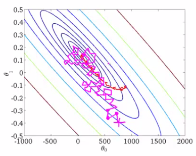
The lines of the level of some function are drawn, the minimum we are looking for. The red curve represents the change in weights (in the picture $\ theta_0$ and $\ theta_1$ match $w_0$ and $w_1$ in our example). According to the properties of the gradient, the direction of change at each point will be perpendicular to the level lines. With the stochastic approach, at each iteration, the weight changes less predictably, sometimes it even seems that some steps are unsuccessful — they lead away from the cherished minimum — but in the end both procedures converge to about the same solution.

The convergence of a stochastic gradient descent to the same solution as that of a gradient descent is one of the most important facts proved in the theory of optimization. Now in the era of Deep Data and Big Learning, it is often the stochastic version that is simply called gradient descent.

Online approach to learning

A stochastic gradient descent, being one of the optimization methods, provides quite practical guidance for learning classification and regression algorithms on large samples - up to hundreds of gigabytes (depending on the available memory).

In the case of paired regression, which we have considered, a training set can be stored on disk. $(X, y)$ and, without loading it into RAM (it may simply not fit), read objects one by one and update the weights:

b e g i n a r r a y r c l w_{0}^{(t + 1)} = w_{0}^{(t)} + e t a (y_{i} - w_{0}^{(t)} - ​ ​ w_{1}^{(t)} x_{i}) w_{1}^{(t + 1)} = w_{1}^{(t)} + e t a (y_{i} - w_{0}^{(t)} - ​ ​ w_{1}^{(t)} x_{i}) x_{i} e n d a r r a y

$\ begin {array} {rcl} w_0 ^ {(t + 1)} = w_0 ^ {(t)} + \ eta (y_i - w_0 ^ {(t)} - w_1 ^ {(t)} x_i) \ \ w_1 ^ {(t + 1)} = w_1 ^ {(t)} + \ eta (y_i - w_0 ^ {(t)} - w_1 ^ {(t)} x_i) x_i \ end {array}$

After processing all the objects of the training sample, the functionality that we optimize (a quadratic error in the regression problem or, for example, logistic one in the classification task) will decrease, but often dozens of passes through the sample are needed so that it decreases sufficiently.

Such an approach to learning models is often called online learning, the term appeared even before MOOC became mainstream.

In this article we do not consider many nuances of stochastic optimization (this is a good article on Habré, you can study this topic fundamentally using the book Boyd "Convex Optimization"), we’ll move on to the Vowpal Wabbit library, which can be used to train simple models on huge samples due to stochastic optimization and one more trick - feature hashing, which will be discussed later.

In the Scikit-learn library, classifiers and regressors, trained by stochastic gradient descent, are implemented by the SGDClassifier and SGDRegressor from sklearn.linear_model .

Working with categorical features: Label Encoding, One-Hot Encoding, Hashing trick

Label Encoding

The overwhelming majority of the methods of classification and regression are formulated in terms of Euclidean or metric spaces, that is, they imply the representation of data in the form of real vectors of the same dimension. In real data, however, categorical features that take discrete values, such as yes / no or January / February /.../ December, are not so rare. We will discuss how to work with such data, in particular with the help of linear models, and what to do if there are many categorical signs, and even each has a bunch of unique values.

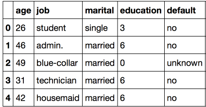
Consider a sample of the UCI bank, in which most of the signs are categorical.

Library Import and Data Load Code

 import warnings warnings.filterwarnings('ignore') import os import re import numpy as np import pandas as pd from sklearn.model_selection import train_test_split from sklearn.linear_model import LogisticRegression from sklearn.metrics import classification_report, accuracy_score from sklearn.metrics import roc_auc_score, roc_curve, confusion_matrix from sklearn.preprocessing import LabelEncoder, OneHotEncoder from sklearn.datasets import fetch_20newsgroups, load_files import pandas as pd from scipy.sparse import csr_matrix import matplotlib.pyplot as plt %matplotlib inline import seaborn as sns df = pd.read_csv('../../data/bank_train.csv') labels = pd.read_csv('../../data/bank_train_target.csv', header=None) df.head()

It is easy to see that quite a few signs in this data set are not represented by numbers. In this form, the data we still do not fit: we can not use the vast majority of the methods available to us.

To find a solution, let's consider the sign of education :

Charting code

 df['education'].value_counts().plot.barh();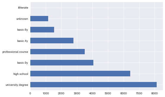

A natural solution to this problem would be to uniquely map each value to a unique number. For example, we could convert university.degree to 0, and basic.9y to 1. This simple operation has to be done often, so the sklearn class is implemented for this task in the sklearn preprocessing module:

The fit method of this class finds all unique values and builds a table to match each category to a certain number, and the transform method directly converts the values into numbers. After fit , a label_encoder field containing all unique values will be available for the classes_ . You can number them and make sure that the conversion is done correctly.

Checking the LabelEncoder conversion

 label_encoder = LabelEncoder() mapped_education = pd.Series(label_encoder.fit_transform(df['education'])) mapped_education.value_counts().plot.barh() print(dict(enumerate(label_encoder.classes_)))

 {0: 'basic.4y', 1: 'basic.6y', 2: 'basic.9y', 3: 'high.school', 4: 'illiterate', 5: 'professional.course', 6: 'university.degree', 7: 'unknown'}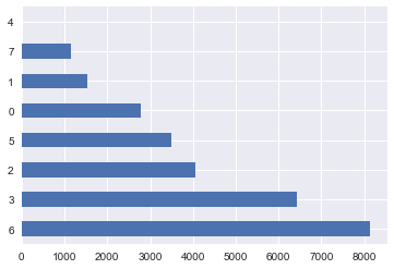

What happens if we have data with other categories? LabelEncoder that it does not know the new category.

Swearing LabelEncoder

 try: label_encoder.transform(df['education'].replace('high.school', 'high_school')) except Exception as e: print('Error:', e)

 Error: y contains new labels: ['high_school']

Thus, when using this approach, we must always be sure that a feature cannot take previously unknown values. We will return to this problem a little later, and now we will replace the entire column of education with the converted one:

We continue the conversion for all columns of type object — this type is specified in pandas for such data.

Code

 categorical_columns = df.columns[df.dtypes == 'object'].union(['education']) for column in categorical_columns: df[column] = label_encoder.fit_transform(df[column]) df.head()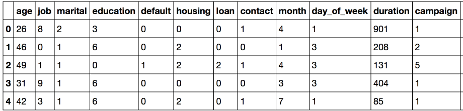

The main problem with this representation is that the numeric code created a Euclidean representation for the data.

For example, we implicitly introduced algebra over the values of the work — we can subtract the work of client 1 from the work of client 2. Of course, this operation has no meaning. But it is precisely on this that the proximity metrics of objects are based, which makes it meaningless to use the nearest-neighbor method on data in this form. Similarly, the use of linear models will make no sense. Let's see how the logistic regression will work on such data and make sure that nothing good happens.

Logistics Regression Training

 def logistic_regression_accuracy_on(dataframe, labels): features = dataframe.as_matrix() train_features, test_features, train_labels, test_labels = \ train_test_split(features, labels) logit = LogisticRegression() logit.fit(train_features, train_labels) return classification_report(test_labels, logit.predict(test_features)) print(logistic_regression_accuracy_on(df[categorical_columns], labels))

  precision recall f1-score support 0 0.89 1.00 0.94 6159 1 0.00 0.00 0.00 740 avg / total 0.80 0.89 0.84 6899

In order for us to apply linear models on such data, we need another method called One-Hot Encoding.

One-Hot Encoding

Suppose that some feature can take 10 different values. In this case, One Hot Encoding involves the creation of 10 features, all of which are zero except for one . At the position corresponding to the numerical value of the attribute we put 1.

This technique is implemented in sklearn.preprocessing in the OneHotEncoder class. By default, OneHotEncoder converts data into a sparse matrix, so as not to consume memory to store multiple zeros. However, in this example, the size of the data is not a problem for us, so we will use a "dense" representation.

Code

 onehot_encoder = OneHotEncoder(sparse=False) encoded_categorical_columns = pd.DataFrame(onehot_encoder.fit_transform(df[categorical_columns])) encoded_categorical_columns.head()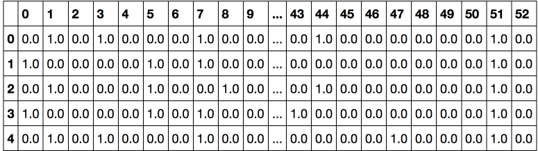

We got 53 columns - these are the numbers of different unique values that categorical columns of the original sample can accept. The data transformed using One-Hot Encoding begins to make sense for the linear model - the accuracy of class 1 (who confirmed the credit) was 61%, completeness - 17%.

Logistic Regression Training

 print(logistic_regression_accuracy_on(encoded_categorical_columns, labels))

  precision recall f1-score support 0 0.90 0.99 0.94 6126 1 0.61 0.17 0.27 773 avg / total 0.87 0.89 0.87 6899

Hashing tricks (Hashing trick)

Real data may turn out to be much more dynamic, and we can not always expect that categorical signs will not take on new values. All this greatly complicates the use of already trained models on new data. In addition, LabelEncoder implies a preliminary analysis of the entire sample and storage of the constructed maps in memory, which makes it difficult to work in big data mode.

To solve these problems, there is a simpler approach to vectoring categorical features based on hashing, known as hashing trick.

Hash functions can help us in the task of searching for unique codes for different values of a feature, for example:

 for s in ('university.degree', 'high.school', 'illiterate'): print(s, '->', hash(s))

 university.degree -> -5073140156977989958 high.school -> -8439808450962279468 illiterate -> -2719819637717010547

Negative values that are so large in magnitude do not suit us. Restrict the range of hash functions:

 hash_space = 25 for s in ('university.degree', 'high.school', 'illiterate'): print(s, '->', hash(s) % hash_space)

 university.degree -> 17 high.school -> 7 illiterate -> 3

Imagine that in our sample there is a single student who was called on Monday, then his feature vector will be formed similarly to One-Hot Encoding, but in a single fixed-size space for all features:

 hashing_example = pd.DataFrame([{i: 0.0 for i in range(hash_space)}]) for s in ('job=student', 'marital=single', 'day_of_week=mon'): print(s, '->', hash(s) % hash_space) hashing_example.loc[0, hash(s) % hash_space] = 1 hashing_example

 job=student -> 6 marital=single -> 8 day_of_week=mon -> 16

It is worth noting that in this example, not only the values of the signs, but the pairs of the name of the attribute + the value of the attribute were hashed. This is necessary to divide the same values of different signs among themselves, for example:

 assert hash('no') == hash('no') assert hash('housing=no') != hash('loan=no')

Can a hash function collide, that is, a match for two different values? It is not difficult to prove that, with a sufficient amount of hashing space, this rarely happens, but even in cases where this happens, it will not lead to a significant deterioration in the quality of classification or regression.

You might ask, “what the hell is going on?”, And it seems that common sense suffers when hashing signs. Perhaps, but this heuristic is, in fact, the only approach to working with categorical features that have many unique meanings. Moreover, this technique has proven itself well in terms of results in practice. More information about the hashing of signs (learning to hash) can be found in this review, as well as in the materials of Evgeny Sokolov.

Vowpal Wabbit Library

Vowpal Wabbit (VW) is one of the most widely used libraries in the industry. It is distinguished by high speed of work and support of a large number of different training modes. Of particular interest for large and high-dimensional data is online learning - the strongest side of the library. Hash features are also implemented, and Vowpal Wabbit is great for working with text data.

The main interface for working with VW is the shell. Vowpal Wabbit reads data from a file or standard input (stdin) in a format that looks like this:

[Label] [Importance] [Tag]|Namespace Features |Namespace Features ... |Namespace Features

Namespace=String[:Value]

Features=(String[:Value] )*

where [] denotes optional elements, and (...) * means to repeat indefinitely.

A label is a number, the "correct" answer. In the case of classification, it usually takes the value 1 / -1, and in the case of regression, some real number
Importance is a number and is responsible for the weight of the example when learning. This allows you to deal with the problem of unbalanced data, we have studied earlier
A tag is some string without spaces and is responsible for some "name" of the example, which is preserved when the response is predicted. In order to separate the Tag from the Importance, it is better to start the Tag with the symbol '.
Namespace is used to create separate feature spaces. Namespace arguments are named after the first letter; this should be taken into account when choosing their names.
Features are directly object attributes inside Namespace . The default signs have a weight of 1.0, but it can be overridden, for example feature: 0.1.

For example, the following line fits this format:

 1 1.0 |Subject WHAT car is this |Organization University of Maryland:0.5 College Park

VW is an excellent tool for working with text data. We verify this with a sample of 20newsgroups containing news from 20 different thematic ezines.

News. Binary classification

 newsgroups = fetch_20newsgroups('../../data/news_data')

Each news item relates to one of 20 topics: alt.atheism, comp.graphics, comp.os.ms-windows.misc, comp.sys.ibm.pc.hardware, comp.sys.mac.hardware, comp.windows.x , misc.forsalerec.autos, rec.motorcycles, rec.sport.baseball, rec.sport.hockey, sci.crypt, sci.electronics, sci.med, sci.space, soc.religion.christian, talk.politics.guns , talk.politics.mideast, talk.politics.misc, talk.religion.misc.

Consider the first text document of this collection:

Code

 text = newsgroups['data'][0] target = newsgroups['target_names'][newsgroups['target'][0]] print('-----') print(target) print('-----') print(text.strip()) print('----')

 ----- rec.autos ----- From: lerxst@wam.umd.edu (where's my thing) Subject: WHAT car is this!? Nntp-Posting-Host: rac3.wam.umd.edu Organization: University of Maryland, College Park Lines: 15 I was wondering if anyone out there could enlighten me on this car I saw the other day. It was a 2-door sports car, looked to be from the late 60s/ early 70s. It was called a Bricklin. The doors were really small. In addition, the front bumper was separate from the rest of the body. This is all I know. If anyone can tellme a model name, engine specs, years of production, where this car is made, history, or whatever info you have on this funky looking car, please e-mail. Thanks, - IL ---- brought to you by your neighborhood Lerxst ---- ----

We give data to the format Vowpal Wabbit, while leaving only words not shorter than 3 characters. Here we do not perform many important procedures in the analysis of texts (stemming and lemmatization), but, as we shall see, the problem will be well solved.

Code

 def to_vw_format(document, label=None): return str(label or '') + ' |text ' + ' '.join(re.findall('\w{3,}', document.lower())) + '\n' to_vw_format(text, 1 if target == 'rec.autos' else -1)

 '1 |text from lerxst wam umd edu where thing subject what car this nntp posting host rac3 wam umd edu organization university maryland college park lines was wondering anyone out there could enlighten this car saw the other day was door sports car looked from the late 60s early 70s was called bricklin the doors were really small addition the front bumper was separate from the rest the body this all know anyone can tellme model name engine specs years production where this car made history whatever info you have this funky looking car please mail thanks brought you your neighborhood lerxst\n'

We split the sample into a training and test and write to the file the documents converted in this way. We will consider the document positive if it relates to the mailing list about cars rec.autos . So we will build a model that distinguishes the news about cars from the rest.

Code

 all_documents = newsgroups['data'] all_targets = [1 if newsgroups['target_names'][target] == 'rec.autos' else -1 for target in newsgroups['target']]

 train_documents, test_documents, train_labels, test_labels = \ train_test_split(all_documents, all_targets, random_state=7) with open('../../data/news_data/20news_train.vw', 'w') as vw_train_data: for text, target in zip(train_documents, train_labels): vw_train_data.write(to_vw_format(text, target)) with open('../../data/news_data/20news_test.vw', 'w') as vw_test_data: for text in test_documents: vw_test_data.write(to_vw_format(text))

Run Vowpal Wabbit on the generated file. We solve the classification problem; therefore, we define the loss function in the hinge value (linear SVM). We will save the constructed model to the appropriate file 20news_model.vw .

 !vw -d ../../data/news_data/20news_train.vw \ --loss_function hinge -f ../../data/news_data/20news_model.vw

 final_regressor = ../../data/news_data/20news_model.vw Num weight bits = 18 learning rate = 0.5 initial_t = 0 power_t = 0.5 using no cache Reading datafile = ../../data/news_data/20news_train.vw num sources = 1 average since example example current current current loss last counter weight label predict features 1.000000 1.000000 1 1.0 -1.0000 0.0000 157 0.911276 0.822551 2 2.0 -1.0000 -0.1774 159 0.605793 0.300311 4 4.0 -1.0000 -0.3994 92 0.419594 0.233394 8 8.0 -1.0000 -0.8167 129 0.313998 0.208402 16 16.0 -1.0000 -0.6509 108 0.196014 0.078029 32 32.0 -1.0000 -1.0000 115 0.183158 0.170302 64 64.0 -1.0000 -0.7072 114 0.261046 0.338935 128 128.0 1.0000 -0.7900 110 0.262910 0.264774 256 256.0 -1.0000 -0.6425 44 0.216663 0.170415 512 512.0 -1.0000 -1.0000 160 0.176710 0.136757 1024 1024.0 -1.0000 -1.0000 194 0.134541 0.092371 2048 2048.0 -1.0000 -1.0000 438 0.104403 0.074266 4096 4096.0 -1.0000 -1.0000 644 0.081329 0.058255 8192 8192.0 -1.0000 -1.0000 174 finished run number of examples per pass = 8485 passes used = 1 weighted example sum = 8485.000000 weighted label sum = -7555.000000 average loss = 0.079837 best constant = -1.000000 best constant's loss = 0.109605 total feature number = 2048932

The model is trained. VW displays a lot of useful information in the course of training (nevertheless, it can be redeemed by setting the parameter --quiet). Details of the diagnostic information is disassembled in the VW documentation on GitHub - here . Please note that the average loss decreased during the iterations. To calculate the loss function, VW uses examples that have not yet been viewed; therefore, as a rule, this estimate is correct. Apply the trained model to the test set, saving the predictions to a file using the -p option:

 !vw -i ../../data/news_data/20news_model.vw -t -d ../../data/news_data/20news_test.vw \ -p ../../data/news_data/20news_test_predictions.txt

 only testing predictions = ../../data/news_data/20news_test_predictions.txt Num weight bits = 18 learning rate = 0.5 initial_t = 0 power_t = 0.5 using no cache Reading datafile = ../../data/news_data/20news_test.vw num sources = 1 average since example example current current current loss last counter weight label predict features 0.000000 0.000000 1 1.0 unknown 1.0000 349 0.000000 0.000000 2 2.0 unknown -1.0000 50 0.000000 0.000000 4 4.0 unknown -1.0000 251 0.000000 0.000000 8 8.0 unknown -1.0000 237 0.000000 0.000000 16 16.0 unknown -0.8978 106 0.000000 0.000000 32 32.0 unknown -1.0000 964 0.000000 0.000000 64 64.0 unknown -1.0000 261 0.000000 0.000000 128 128.0 unknown 0.4621 82 0.000000 0.000000 256 256.0 unknown -1.0000 186 0.000000 0.000000 512 512.0 unknown -1.0000 162 0.000000 0.000000 1024 1024.0 unknown -1.0000 283 0.000000 0.000000 2048 2048.0 unknown -1.0000 104 finished run number of examples per pass = 2829 passes used = 1 weighted example sum = 2829.000000 weighted label sum = 0.000000 average loss = 0.000000 total feature number = 642215

, AUC ROC-:

Code

 with open('../../data/news_data/20news_test_predictions.txt') as pred_file: test_prediction = [float(label) for label in pred_file.readlines()] auc = roc_auc_score(test_labels, test_prediction) roc_curve = roc_curve(test_labels, test_prediction) with plt.xkcd(): plt.plot(roc_curve[0], roc_curve[1]); plt.plot([0,1], [0,1]) plt.xlabel('FPR'); plt.ylabel('TPR'); plt.title('test AUC = %f' % (auc)); plt.axis([-0.05,1.05,-0.05,1.05]);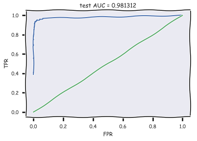

AUC .

News.

, , . Vowpal Wabbit – , 1 K, K – ( – 20). LabelEncoder, ( LabelEncoder 0 K-1).

Code

 all_documents = newsgroups['data'] topic_encoder = LabelEncoder() all_targets_mult = topic_encoder.fit_transform(newsgroups['target']) + 1

, , train_labels_mult test_labels_mult – 1 20.

Code

 train_documents, test_documents, train_labels_mult, test_labels_mult = \ train_test_split(all_documents, all_targets_mult, random_state=7) with open('../../data/news_data/20news_train_mult.vw', 'w') as vw_train_data: for text, target in zip(train_documents, train_labels_mult): vw_train_data.write(to_vw_format(text, target)) with open('../../data/news_data/20news_test_mult.vw', 'w') as vw_test_data: for text in test_documents: vw_test_data.write(to_vw_format(text))

Vowpal Wabbit , oaa ( "one against all"), . , , ( – Vowpal Wabbit):

(-l, 0.5) –
(--power_t, 0.5) – , ,
(--loss_function) – , , .
(-l1) – , VW , , $10^{-20}.$

Vowpal Wabbit Hyperopt. Python 2. .

Code

 %%time !vw --oaa 20 ../../data/news_data/20news_train_mult.vw \ -f ../../data/news_data/20news_model_mult.vw --loss_function=hinge

 final_regressor = ../../data/news_data/20news_model_mult.vw Num weight bits = 18 learning rate = 0.5 initial_t = 0 power_t = 0.5 using no cache Reading datafile = ../../data/news_data/20news_train_mult.vw num sources = 1 average since example example current current current loss last counter weight label predict features 1.000000 1.000000 1 1.0 15 1 157 1.000000 1.000000 2 2.0 2 15 159 1.000000 1.000000 4 4.0 15 10 92 1.000000 1.000000 8 8.0 16 15 129 1.000000 1.000000 16 16.0 13 12 108 0.937500 0.875000 32 32.0 2 9 115 0.906250 0.875000 64 64.0 16 16 114 0.867188 0.828125 128 128.0 8 4 110 0.816406 0.765625 256 256.0 7 15 44 0.646484 0.476562 512 512.0 13 9 160 0.502930 0.359375 1024 1024.0 3 4 194 0.388672 0.274414 2048 2048.0 1 1 438 0.300293 0.211914 4096 4096.0 11 11 644 0.225098 0.149902 8192 8192.0 5 5 174 finished run number of examples per pass = 8485 passes used = 1 weighted example sum = 8485.000000 weighted label sum = 0.000000 average loss = 0.222392 total feature number = 2048932 CPU times: user 7.97 ms, sys: 13.9 ms, total: 21.9 ms Wall time: 378 ms

 %%time !vw -i ../../data/news_data/20news_model_mult.vw -t \ -d ../../data/news_data/20news_test_mult.vw \ -p ../../data/news_data/20news_test_predictions_mult.txt

 only testing predictions = ../../data/news_data/20news_test_predictions_mult.txt Num weight bits = 18 learning rate = 0.5 initial_t = 0 power_t = 0.5 using no cache Reading datafile = ../../data/news_data/20news_test_mult.vw num sources = 1 average since example example current current current loss last counter weight label predict features 1.000000 1.000000 1 1.0 unknown 8 349 1.000000 1.000000 2 2.0 unknown 6 50 1.000000 1.000000 4 4.0 unknown 18 251 1.000000 1.000000 8 8.0 unknown 18 237 1.000000 1.000000 16 16.0 unknown 4 106 1.000000 1.000000 32 32.0 unknown 15 964 1.000000 1.000000 64 64.0 unknown 4 261 1.000000 1.000000 128 128.0 unknown 8 82 1.000000 1.000000 256 256.0 unknown 10 186 1.000000 1.000000 512 512.0 unknown 1 162 1.000000 1.000000 1024 1024.0 unknown 11 283 1.000000 1.000000 2048 2048.0 unknown 14 104 finished run number of examples per pass = 2829 passes used = 1 weighted example sum = 2829.000000 weighted label sum = 0.000000 average loss = 1.000000 total feature number = 642215 CPU times: user 4.28 ms, sys: 9.65 ms, total: 13.9 ms Wall time: 166 ms

 with open('../../data/news_data/20news_test_predictions_mult.txt') as pred_file: test_prediction_mult = [float(label) for label in pred_file.readlines()]

 accuracy_score(test_labels_mult, test_prediction_mult)

87%.

, , .

Code

 M = confusion_matrix(test_labels_mult, test_prediction_mult) for i in np.where(M[0,:] > 0)[0][1:]: print(newsgroups['target_names'][i], M[0,i], )

 rec.autos 1 rec.sport.baseball 1 sci.med 1 soc.religion.christian 3 talk.religion.misc 5

: rec.autos, rec.sport.baseball, sci.med, soc.religion.christian talk.religion.misc.

IMDB

, IMDB. , Vowpal Wabbit.

load_files sklearn.datasets . imdb_reviews ( train test ). – 100 . . 12500 . (, ) .

Code

 #     path_to_movies = '/Users/y.kashnitsky/Yandex.Disk.localized/ML/data/imdb_reviews/' reviews_train = load_files(os.path.join(path_to_movies, 'train')) text_train, y_train = reviews_train.data, reviews_train.target

 print("Number of documents in training data: %d" % len(text_train)) print(np.bincount(y_train))

 Number of documents in training data: 25000 [12500 12500]

 reviews_test = load_files(os.path.join(path_to_movies, 'test')) text_test, y_test = reviews_test.data, reviews_train.target print("Number of documents in test data: %d" % len(text_test)) print(np.bincount(y_test))

 Number of documents in test data: 25000 [12500 12500]

 "Zero Day leads you to think, even re-think why two boys/young men would do what they did - commit mutual suicide via slaughtering their classmates. It captures what must be beyond a bizarre mode of being for two humans who have decided to withdraw from common civility in order to define their own/mutual world via coupled destruction.<br /><br />It is not a perfect movie but given what money/time the filmmaker and actors had - it is a remarkable product. In terms of explaining the motives and actions of the two young suicide/murderers it is better than 'Elephant' - in terms of being a film that gets under our 'rationalistic' skin it is a far, far better film than almost anything you are likely to see. <br /><br />Flawed but honest with a terrible honesty."

. :

 'Words can\'t describe how bad this movie is. I can\'t explain it by writing only. You have too see it for yourself to get at grip of how horrible a movie really can be. Not that I recommend you to do that. There are so many clich\xc3\xa9s, mistakes (and all other negative things you can imagine) here that will just make you cry. To start with the technical first, there are a LOT of mistakes regarding the airplane. I won\'t list them here, but just mention the coloring of the plane. They didn\'t even manage to show an airliner in the colors of a fictional airline, but instead used a 747 painted in the original Boeing livery. Very bad. The plot is stupid and has been done many times before, only much, much better. There are so many ridiculous moments here that i lost count of it really early. Also, I was on the bad guys\' side all the time in the movie, because the good guys were so stupid. "Executive Decision" should without a doubt be you\'re choice over this one, even the "Turbulence"-movies are better. In fact, every other movie in the world is better than this one.'

to_vw_format . ( movie_reviews_train.vw ), ( movie_reviews_valid.vw ) ( movie_reviews_test.vw ) Vowpal Wabbit. 70% , 30% – .

Code

 train_share = int(0.7 * len(text_train)) train, valid = text_train[:train_share], text_train[train_share:] train_labels, valid_labels = y_train[:train_share], y_train[train_share:] with open('../../data/movie_reviews_train.vw', 'w') as vw_train_data: for text, target in zip(train, train_labels): vw_train_data.write(to_vw_format(str(text), 1 if target == 1 else -1)) with open('../../data/movie_reviews_valid.vw', 'w') as vw_train_data: for text, target in zip(valid, valid_labels): vw_train_data.write(to_vw_format(str(text), 1 if target == 1 else -1)) with open('../../data/movie_reviews_test.vw', 'w') as vw_test_data: for text in text_test: vw_test_data.write(to_vw_format(str(text)))

Vowpal Wabbit :

-d, (. .vw )
--loss_function – hinge ( )
-f – , ( .vw)

 !vw -d ../../data/movie_reviews_train.vw \ --loss_function hinge -f movie_reviews_model.vw --quiet

Vowpal Wabbit, :

-i – (. .vw)
-t -d – (. .vw)
-p – txt-,

 !vw -i movie_reviews_model.vw -t -d ../../data/movie_reviews_valid.vw \ -p movie_valid_pred.txt --quiet

ROC AUC. , VW +1. [-1, 1], (0 1) , . AUC 88.5% – 94.2% – .

Code

 with open('movie_valid_pred.txt') as pred_file: valid_prediction = [float(label) for label in pred_file.readlines()] print("Accuracy: {}".format(round(accuracy_score(valid_labels, [int(pred_prob > 0) for pred_prob in valid_prediction]), 3))) print("AUC: {}".format(round(roc_auc_score(valid_labels, valid_prediction), 3)))

 !vw -i movie_reviews_model.vw -t -d ../../data/movie_reviews_test.vw \ -p movie_test_pred.txt --quiet

 with open('movie_test_pred.txt') as pred_file: test_prediction = [float(label) for label in pred_file.readlines()] print("Accuracy: {}".format(round(accuracy_score(y_test, [int(pred_prob > 0) for pred_prob in test_prediction]), 3))) print("AUC: {}".format(round(roc_auc_score(y_test, test_prediction), 3)))

 Accuracy: 0.88 AUC: 0.94

. – 89% AUC 95% .

Code

 !vw -d ../../data/movie_reviews_train.vw \ --loss_function hinge --ngram 2 -f movie_reviews_model2.vw --quiet

 !vw -i movie_reviews_model2.vw -t -d ../../data/movie_reviews_valid.vw \ -p movie_valid_pred2.txt --quiet

 with open('movie_valid_pred2.txt') as pred_file: valid_prediction = [float(label) for label in pred_file.readlines()] print("Accuracy: {}".format(round(accuracy_score(valid_labels, [int(pred_prob > 0) for pred_prob in valid_prediction]), 3))) print("AUC: {}".format(round(roc_auc_score(valid_labels, valid_prediction), 3)))

 Accuracy: 0.894 AUC: 0.954

 !vw -i movie_reviews_model2.vw -t -d ../../data/movie_reviews_test.vw \ -p movie_test_pred2.txt --quiet

 with open('movie_test_pred2.txt') as pred_file: test_prediction2 = [float(label) for label in pred_file.readlines()] print("Accuracy: {}".format(round(accuracy_score(y_test, [int(pred_prob > 0) for pred_prob in test_prediction2]), 3))) print("AUC: {}".format(round(roc_auc_score(y_test, test_prediction2), 3)))

 Accuracy: 0.888 AUC: 0.952

StackOverflow

, Vowpal Wabbit . 10 StackOverflow – , 10 , . , .

10, 10 : 10 , 10 .

 #     PATH_TO_DATA = '/Users/y.kashnitsky/Documents/Machine_learning/org_mlcourse_ai/private/stackoverflow_hw/' !du -hs $PATH_TO_DATA/stackoverflow_10mln_*.vw

 1,4G /Users/y.kashnitsky/Documents/Machine_learning/org_mlcourse_ai/private/stackoverflow_hw//stackoverflow_10mln_test.vw 3,3G /Users/y.kashnitsky/Documents/Machine_learning/org_mlcourse_ai/private/stackoverflow_hw//stackoverflow_10mln_train.vw 1,9G /Users/y.kashnitsky/Documents/Machine_learning/org_mlcourse_ai/private/stackoverflow_hw//stackoverflow_10mln_train_part.vw 1,4G /Users/y.kashnitsky/Documents/Machine_learning/org_mlcourse_ai/private/stackoverflow_hw//stackoverflow_10mln_valid.vw

, Vowpal Wabbit. 10 10 , .

 10 | i ve got some code in window scroll that checks if an element is visible then triggers another function however only the first section of code is firing both bits of code work in and of themselves if i swap their order whichever is on top fires correctly my code is as follows fn isonscreen function use strict var win window viewport top win scrolltop left win scrollleft bounds this offset viewport right viewport left + win width viewport bottom viewport top + win height bounds right bounds left + this outerwidth bounds bottom bounds top + this outerheight return viewport right lt bounds left viewport left gt bounds right viewport bottom lt bounds top viewport top gt bounds bottom window scroll function use strict var load_more_results ajax load_more_results isonscreen if load_more_results true loadmoreresults var load_more_staff ajax load_more_staff isonscreen if load_more_staff true loadmorestaff what am i doing wrong can you only fire one event from window scroll i assume not

(3.3 ) Vowpal Wabbit :

-oaa 10 – , 10
-d –
-f – ,
-b 28 – 28 , $2^{28}$ , , ( - , )
random seed

 %%time !vw --oaa 10 -d $PATH_TO_DATA/stackoverflow_10mln_train.vw \ -f vw_model1_10mln.vw -b 28 --random_seed 17 --quiet

 CPU times: user 592 ms, sys: 220 ms, total: 813 ms Wall time: 39.9 s

40 , 14 , – 92%. , . .

 %%time !vw -t -i vw_model1_10mln.vw \ -d $PATH_TO_DATA/stackoverflow_10mln_test.vw \ -p vw_valid_10mln_pred1.csv --random_seed 17 --quiet

 CPU times: user 198 ms, sys: 83.1 ms, total: 281 ms Wall time: 14.1 s

 import os import numpy as np from sklearn.metrics import accuracy_score vw_pred = np.loadtxt('vw_valid_10mln_pred1.csv') test_labels = np.loadtxt(os.path.join(PATH_TO_DATA, 'stackoverflow_10mln_test_labels.txt')) accuracy_score(test_labels, vw_pred)

 0.91868709729356979

, .

- . Jupyter notebook - ( ).

useful links

Open Machine Learning Course. Topic 8. Vowpal Wabbit: Fast Learning with Gigabytes of Data
: ( ), ( ), Vowpal Wabbit
"Numeric Computation" "Deep Learning"
Vowpal Wabbit GitHub
, (VW) Hadoop-
VW
VW hyperopt

Jupyter GitHub- .

Source: https://habr.com/ru/post/326418/

All Articles

Open machine learning course. Topic 8. Gigabyte training with Vowpal Wabbit

Plan

Stochastic Gradient Descent and Online Learning Approach

Stochastic Gradient Descent

Online approach to learning

Working with categorical features: Label Encoding, One-Hot Encoding, Hashing trick

Label Encoding

One-Hot Encoding

Hashing tricks (Hashing trick)

Vowpal Wabbit Library

News. Binary classification

News.

IMDB

StackOverflow

useful links

More articles: