The logic of consciousness. Part 12. The search for patterns. Combinatorial space

Poetry - the same mining radium.
In gram extraction, in the years of labor.
You harass a single word for
Thousands of tons of verbal ore.
But how sizzling these burning words
Next to the decay of raw words.
These words set in motion
Thousands of years of millions of hearts.

Vladimir Mayakovsky

Let me remind you that our immediate task is to show a universal generalization algorithm. Such a generalization should satisfy all the requirements formulated earlier in the tenth part . In addition, it should be free from the traditional for many methods of machine learning deficiencies (combinatorial explosion, retraining, convergence to a local minimum, the stability-plasticity dilemma, and the like). Moreover, the mechanism of such a generalization should not contradict our knowledge of the work of the real neurons of the living brain.
')
We take one more step towards universal generalization. We describe the idea of ​​a combinatorial space and how this space helps to look for patterns and thereby solve the problem of learning with a teacher.

The task of shifting the text line

Now we will show how very difficult it is to solve a very simple task. We will learn to move an arbitrary text string one position.

Suppose we have a long text. We consistently read it from beginning to end. In one step of reading, we shift one character. Suppose that we have a sliding window with a width of N characters, and at each moment of time only a fragment of text is available that fits into this window. We introduce a cyclic position identifier (described at the end of the fourth part ), indicating the position of the characters in the text. The period of the identifier is denoted by K. An example of the text with the imposed position identifier and the scanning window is shown in the figure below.


Fragment of the text. Numbers indicate cyclic position identifier. Period id K = 10. Vertical lines highlight one of the positions of the sliding window. Window size N = 6

The basic idea of ​​this view is that if the window size N is less than the period of the identifier K, then the set of “letter-position identifier” pairs allows you to uniquely record a string inside a sliding window. Earlier, we mentioned a similar recording method when we talked about how to encode audio information. Substitute instead of the letters codes of some conditional phonemes, and you get a sound track.

We introduce a system of concepts that allows us to describe everything that appears in a sliding window. For simplicity, we will not make a difference between uppercase and lowercase letters and will not take punctuation marks into account. Since potentially any letter can meet us in any position, we will need all possible combinations of letters and positions, that is, 26 x K concepts. Conventionally, these concepts can be designated as

{a0, a1 ⋯ a (K-1), b0, b1 b (K-1), z0, z1 z (K-1)}

We can record any state of a sliding window as an enumeration of relevant concepts. So for the window shown in the figure above, it will be

{s1, w3, e4, d6}

Let's compare to each concept a certain discharged binary code. For example, if you take a code length of 256 bits and allocate 8 bits to encode one concept, then the encoding of the letter “a” in different positions will look like the one shown in the figure below. Let me remind you that the codes are chosen randomly, and their bits can be repeated, that is, the same bits can be common to several codes.


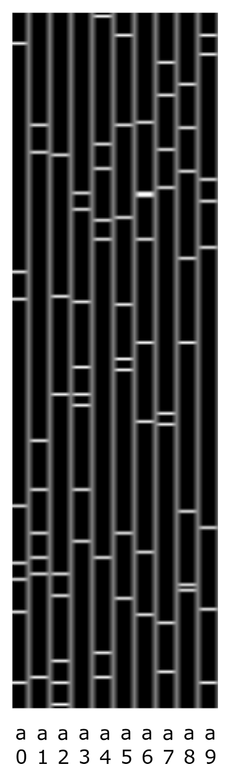
An example of the codes of the letter a in positions from 0 to 9. Binary vectors are shown vertically, units are marked with horizontal light lines.

Create a binary fragment code by the logical addition of the codes of its concepts. As previously stated, such a binary fragment code will have the properties of a Bloom filter. If the bit depth of the binary array is sufficiently high, then with a sufficiently high accuracy, the inverse transformation can be performed and a set of initial concepts can be obtained from the fragment code.

The figure below shows an example of how the concept codes and the summary fragment code for the previous example will look like.

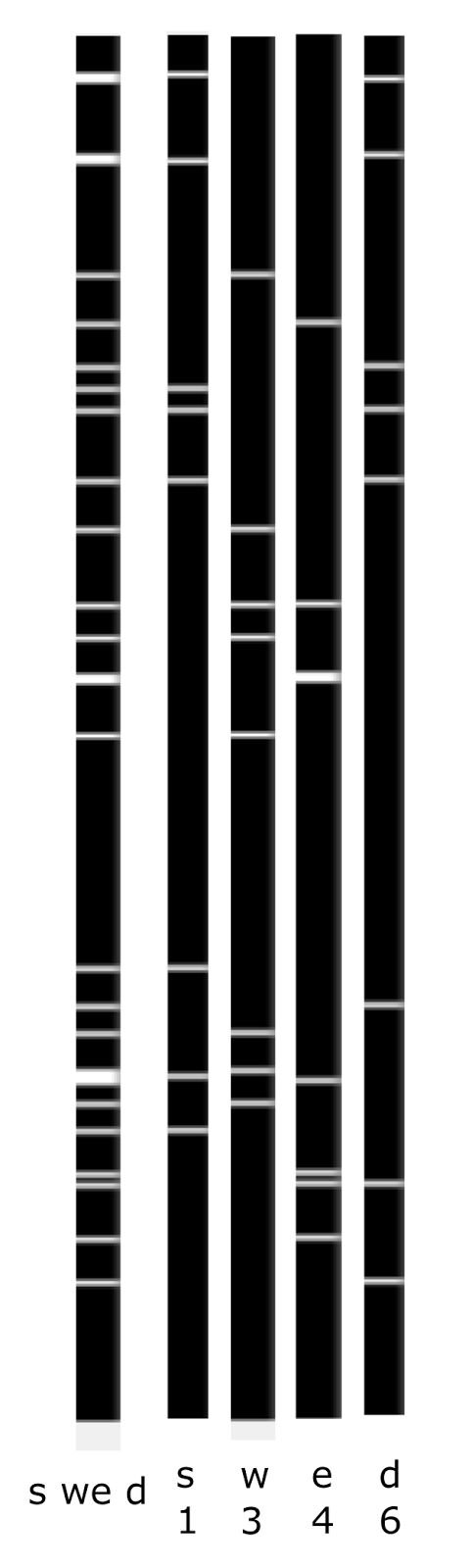
Example of adding binary concept codes to fragment code

A description made in this way stores not only the set of letters of a fragment of text, but also their sequence. However, both the set of concepts and the summary code of this sequence depend on the position in which the cyclic identifier was at the time when the sequence appeared in the text. The figure below shows an example of how the description of the same piece of text depends on the initial position of the cyclic identifier.


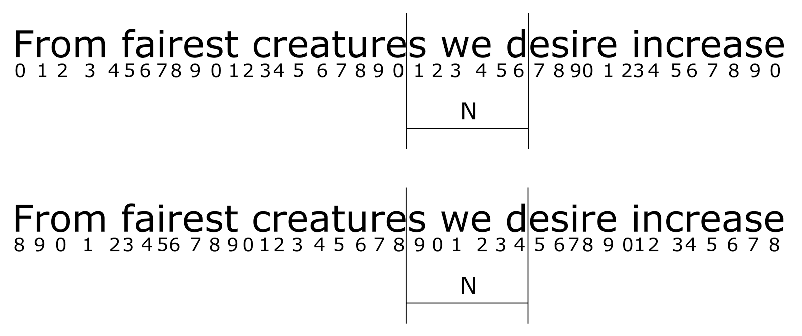
Change text encoding at different initial offset

The first case will correspond to the description

{s1, w3, e4, d6}

The second case will be recorded as

{s9, w1, e2, d4}

As a result, the text is the same, but a completely different set of concepts and, accordingly, a completely different binary code describing it.

Here we come to what was talked about so much in the previous parts . Variants obtained by shifting the text are possible interpretations of the same information. In this context, all possible offset options are used. And although the essence of information is unchanged, its external form, that is, description through a set of concepts or through its binary representation, changes from context to context, that is, in our case, with each change of the initial position.

To be able to compare text fragments invariant to their displacement, it is necessary to introduce the space of displacement contexts. For this, you need K contexts. Each context will correspond to one of the possible initial offset options.

Recall that contexts are determined by the rules of contextual transformations. In each context, a set of rules is defined regarding how concepts change in this context.

Contextual transformations in the case of text will be the rules for changing concepts when moving to an appropriate context shift. For example, for a context with zero offset, the transition rules will be transitions into themselves

a0 → a0, a2 → a2 ⋯ z (K-1) → z (K-1)

For a context with an offset of 8 positions with a ring identifier length K = 10, which corresponds to the bottom line of the example in the figure above, the rules will be
a0 → a8, a1 → a9, a2 → a0 z9 → z7

With such rules in context with an offset of 8, the window description from the first line of the example will go to the window description from the second line, which, in fact, is quite obvious and without much explanation.

{s1, w3, e4, d6} → {s9, w1, e2, d4}

In our case, contexts, in fact, perform a variation of the offset of the text line over all possible positions of the ring identifier. As a result, if the two lines coincide or are similar to each other, but are shifted one relative to the other, then there will always be a context that levels this shift.

Later we will develop the thought about contexts in detail, now we will be interested in one particular, but very important question: how do binary descriptive codes change as we move from one context to another?

In our example, we have the text and we know the positions of the letters. Having set the required offset, we can always recalculate the positions of the letters and get a new description. It is not difficult to calculate the binary codes for the source and offset states. For example, the figure below shows how the code of the string “arkad” at zero offset and the code of the same string will look when shifted one position to the right.


Source Line Code and Offsets

Since we have an algorithm for recalculating descriptions, we can easily get any binary source code (in zero context) and code at one position (in the context of "1") for any string. Taking a long text, we can create any number of such examples pertaining to a single offset.

And now let's take the generated examples and imagine that we have a black box. There is a binary description at the input, there is a binary description at the output, but we do not know anything about the nature of the input description, nor about the rules by which the conversion occurs. Can we reproduce the work of this black box?

We have come to the classic task of learning with a teacher. There is a training sample and it is required to reproduce the internal logic that relates the input and output data.

Such a statement of the problem is typical for situations that the brain often encounters when solving the issues of contextual transformations. For example, in the last part it was described how the retina forms binary codes corresponding to the visual picture. Eye movements are constantly creating learning examples. Since the movements are very fast, we can assume that we see the same scene, but only in different contexts of displacement. Thus, the brain receives the source code of the image and the code into which this image passes in the context of the bias done by the eye. The task of learning visual contexts is the computation of the rules governing visual transformations. Knowledge of these rules allows us to obtain interpretations of the same image simultaneously in different variants of displacements without the need for the eye to physically perform these displacements.

What is the difficulty?

When I studied at the institute, we had a very popular game “Bulls and Cows” . One player makes a four-digit number without repeating, another tries to guess it. The one who tries, calls certain numbers, and the one who informs tells how many bulls are there, that is, guessed numbers standing in his place, and how many cows, numbers that are in the hidden number, but are not where they are supposed to be. The whole point of the game is that the answers of the person who made it up do not give unambiguous information, but create a lot of acceptable options. Each attempt generates such ambiguous information. However, a set of attempts allows you to find the only correct answer.

Something similar is in our problem. Output bits are not random, each of them depends on a specific combination of input bits. But since several concepts can be contained in the input vector, it is not known which bits are responsible for triggering a particular output bit.

Since the bits can be repeated in the concept codes, one input bit says nothing about the output. To judge the output, you want to analyze the combination of several input bits.

Since the same output bit can refer to codes of different concepts, the operation of the output bit does not mean that the same combination of bits appeared at the input, which made this output bit work earlier.

In other words, there is a rather strong uncertainty, both from the input side and from the output side. This uncertainty turns out to be a serious hindrance and makes it difficult to decide too simple. One uncertainty is multiplied by another uncertainty, which results in a combinatorial explosion .

To combat the combinatorial explosion requires "combinatorial scrap." There are two tools that allow in practice to solve complex combinatorial problems. The first is a massively parallel computation. And here it is important not only to have a large number of parallel processors, but also to choose an algorithm that allows you to parallelize the task and load all the available computing power.

The second tool is the principle of limitation. The main method using the principle of boundedness is the method of "random subspaces" . Sometimes combinatorial problems admit a strong limitation of baseline conditions and at the same time retain the hope that even after these limitations enough data will be stored in the data so that the required solution can be found. There are many options for limiting initial conditions. Not all of them can be successful. But if, nevertheless, the probability that there are successful variants of limitations, then a complex task can be broken down into a large number of limited problems, each of which is solved much simpler than the initial one.

Combining these two principles, we can construct a solution to our problem.

Combinatorial space

Take an input bit vector and number its bits. Create combinatorial "points". At each point we add a few random bits of the input vector (figure below). Watching the entrance, each of these points will not see the whole picture, but only a small part of it, determined by what bits converged at the selected point. So, in the figure below, the leftmost point with index 0 monitors only bits 1, 6, 10 and 21 of the original input signal. Create such points quite a lot and call them a set of combinatorial spaces.


Combinatorial space

What is the meaning of this space? We assume that the input signal is not random, but contains certain patterns. Regularities can be of two main types. Something in the input description may appear somewhat more often than another. For example, in our case separate letters appear more often than their combinations. With bit coding, this means that certain combinations of bits occur more often than others.

Another type of pattern is when, in addition to the input signal, there is a learning signal accompanying it and something contained in the input signal turns out to be connected with something that is contained in the learning signal. In our case, the active output bits are a reaction to a combination of certain input bits.

If you look for patterns "in the forehead", that is, looking at the entire input and the entire output vectors, then it is not very clear what to do and where to go. If you begin to build hypotheses on the subject of what may depend on, then immediately a combinatorial explosion occurs. The number of possible hypotheses turns out to be monstrous.

The classical method widely used in neural networks is gradient descent. It is important for him to understand which way to go. Usually it is easy when the output target is one. For example, if we want to teach a neural network to write numbers, we show it images of numbers and indicate what kind of numbers she sees. The network understands how and where to go. If we show pictures with several numbers at once and call all these numbers at the same time, without indicating where something is, then the situation becomes much more complicated.

When the points of a combinatorial space are created with a very limited “view” (random subspaces), it turns out that some of the points may be lucky and they will see the pattern if not completely clean, then at least in a significantly purified form. Such a limited view will allow, for example, to make a gradient descent and get an already pure pattern. The probability for a particular point to stumble on a pattern may not be very high, but you can always pick up such a number of points to ensure that any pattern “comes up somewhere.”

Of course, if the dot sizes are made too narrow, that is, the number of bits in points is approximately equal to how many bits are expected in the pattern, then the sizes of the combinatorial space will begin to strive for the number of options for exhaustive search of possible hypotheses, which returns us to the combinatorial explosion. But, fortunately, you can increase the review points, reducing their total number. This reduction is not given free of charge, combinatorics are “transferred to points”, but until a certain point it is not fatal.

Create an output vector. We will simply add several points of combinatorial space to each output bit. What points will be chosen randomly. The number of points falling in one bit will correspond to how many times we want to reduce the combinatorial space. Such an output vector will be a hash function for the state vector of the combinatorial space. How this condition is considered, we will talk a bit later.

In general, for example, as shown in the figure above, the size of the input and output may be different. In our example, with transcoding strings, these dimensions are the same.

Receptor clusters

How to look for patterns in combinatorial space? Each point sees its own fragment of the input vector. If there are a lot of active bits in what she sees, then we can assume that what she sees is a pattern. That is, a set of active bits that falls into a point can be called a hypothesis about the presence of a pattern. Let us remember this hypothesis, that is, we fix a set of active bits visible at a point. In the situation shown in the figure below, it can be seen that bits 1, 6 and 21 should be fixed at point 0.


Catching bits in a cluster

We will call the record of the number of one bit a receptor for this bit. This implies that the receptor monitors the state of the corresponding bit of the input vector and reacts when a unit appears there.

A set of receptors will be called a receptor cluster or a receptive cluster. When an input vector is presented, the cluster receptors react if units are in the corresponding positions of the vector. For a cluster, you can calculate the number of receptors activated.

Since the information is encoded not by individual bits, but by code, the accuracy with which we formulate a hypothesis depends on how many bits we take into the cluster. The article is attached to the text of the program that solves the problem with the recoding of lines. By default, the program has the following settings:

• input vector length - 256 bits;
  
• output vector length - 256 bits;
  
• a single letter is encoded with 8 bits;
  
• line length - 5 characters;
  
• number of displacement contexts - 10;
  
• combinatorial space size - 60000;
  
• the number of bits intersecting at a point is 32;
  
• cluster creation threshold - 6;
  
• The threshold for partial activation of the cluster is 4.
  

With such settings, almost every bit that is in the code of one letter is repeated in the code of another letter, and even in the codes of several letters. Therefore, a single receptor can not reliably indicate the pattern. Two receptors indicate a letter is much better, but they can also indicate a combination of very different letters. You can enter a certain length threshold, starting from which you can fairly reliably judge whether the necessary code fragment is in the cluster.

We introduce a minimum threshold for the number of receptors necessary for the formation of a hypothesis (in the example, it is equal to 6). Let's start learning. We will submit the source code and the code we want to get at the output. For the source code, it is easy to calculate how many active bits fall into each of the points of the combinatorial space. We select only those points that are connected to the active bits of the output code and whose number of active bits of the input code that fall into it will be no less than the threshold for creating the cluster. At such points, create clusters of receptors with corresponding sets of bits. Let's save these clusters exactly in those points where they were created. In order not to create duplicates, we first check that these clusters are unique for these points and the points do not yet contain exactly the same clusters.

Let's say the same in other words. From the output vector, we know which bits should be active. Accordingly, we can choose the points of combinatorial space associated with them. For each such point, we can formulate a hypothesis that what it now sees on the input vector is the pattern that is responsible for the activity of the bit to which this point is connected. We cannot say by example, whether this hypothesis is true or not, but no one is stopping us from proposing.

Training. Memory consolidation

In the process of learning, each new example creates a huge number of hypotheses, most of which are incorrect. We are required to check all these hypotheses and weed out false ones. We can do this by observing whether these hypotheses will be confirmed in the following examples. In addition, creating a new cluster, we remember all the bits that the dot sees, and this, even if there is a pattern, also random bits that got there from other concepts that do not affect our output, and which in our case are noise. Accordingly, it is required not only to confirm or deny that the stored pattern contains the necessary pattern, but also to clear this combination of noise, leaving only the “clean” rule.

There are different approaches to solving the problem. I will describe one of them, not claiming that he is the best. I went through a lot of options, this one bribed me with quality of work and simplicity, but this does not mean that it cannot be improved.

It is convenient to perceive clusters as autonomous computers. If each cluster can test its hypothesis and make decisions independently of the others, then this is very good for potential parallelization of computations. Each cluster of receptors after creation begins an independent life. He monitors the incoming signals, accumulates experience, changes himself and takes if the decision on self-destruction is necessary.

A cluster is a set of bits, about which we assumed that there is a pattern inside it associated with the triggering of the output bit to which the point containing this cluster is connected. If there is a pattern, then most likely it affects only part of the bits, and we do not know in advance which one. Therefore, we will record all the moments when a significant number of receptors are triggered in the cluster (at least 4 in the example). It is possible that in these moments the pattern, if any, manifests itself. When certain statistics accumulate, we will be able to try to determine whether there is something natural in such partial operations of the cluster or not.

An example of statistics is shown in the figure below. A plus at the beginning of the line indicates that at the moment the cluster was partially triggered, the output bit was also active. Cluster bits are formed from the corresponding bits of the input vector.


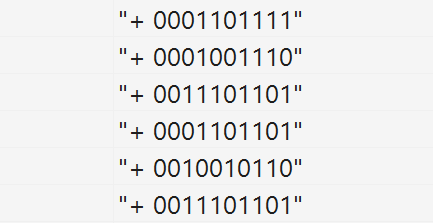
Chronicle of partial receptor cluster response

What should we be interested in in this statistics? It is important to us which bits most often work together. Do not confuse this with the most frequent bits. If we calculate for each bit the frequency of its occurrence and take the most common bits, then it will be averaging, which is not at all what we need. If at the point there are some stable regularities, then at averaging the average between them will be “not regularity”. In our example, it can be seen that 1,2 and 4 lines are similar to each other, also 3.4 and 6 lines are similar. We need to choose one of these patterns, preferably the strongest, and clean it of the extra bits.

The most common combination, which manifests itself as the joint operation of certain bits, is the first main component for this statistic. To calculate the main component, you can use the Hebb filter. For this you can set a vector with unit initial weights. Then get the activity of the cluster, multiplying the weights vector by the current state of the cluster. And then the weights are shifted towards the current state the stronger, the higher this activity. So that the weights do not grow uncontrollably, after changing the weights, they should be normalized, for example, to the maximum value from the weights vector.

This procedure is repeated for all available examples. As a result, the weight vector is increasingly approaching the main component. If there are not enough examples that exist to converge, then you can repeat the process several times with the same examples, gradually reducing the speed of learning.

The basic idea is that as it approaches the main component, the cluster begins to react more and more to samples similar to it and less and less to the others, due to this, learning goes in the right direction faster than “bad” examples try to spoil it. The result of this algorithm after several iterations is shown below.


The result obtained after several iterations of the selection of the first main component

If you now cut the cluster, that is, leave only those receptors that have high weights (for example, above 0.75), then we will get a regularity cleared of unnecessary noise bits. This procedure can be repeated several times as statistics accumulate. As a result, it is possible to understand whether there is any pattern in the cluster, or we have put together a random set of bits. If there is no pattern, then as a result of cutting the cluster, too short a fragment will remain. In this case, such a cluster can be removed as a failed hypothesis.

In addition to trimming the cluster, it is necessary to ensure that the desired pattern is caught. In the original line mixed codes of several letters, each of them is a pattern. Any of these codes can be “caught” by the cluster.But we are only interested in the code of the letter that affects the formation of the output bit. For this reason, most hypotheses will be false and must be rejected. This can be done according to the criteria that the partial or even full operation of the cluster too often will not coincide with the activity of the desired output bit. Such clusters are subject to removal. The process of such control and removal of unnecessary clusters together with their “trimming” can be called memory consolidation.

The process of accumulation of new clusters is quite fast, each new experience forms several thousand new clusters-hypotheses. Training is advisable to carry out the stages with a break for "sleep." When clusters are created a lot of critical, you need to go into the "idle" work. In this mode, the previously recorded experience is scrolled. But this does not create new hypotheses, but only goes to check the old ones. As a result of “sleep,” it is possible to remove a huge percentage of false hypotheses and leave only hypotheses that have been tested. After the “sleep”, the combinatorial space not only turns out to be cleared and ready to receive new information, but also much more confidently is guided by what was learned “yesterday”.

Combinatorial space output

As clusters accumulate statistics and undergo consolidation, clusters will appear that are quite similar to the fact that their hypothesis is either true or close to the truth. We will take such clusters and monitor when they are fully activated, that is, when all the receptors of the cluster are active.

Further from this activity we will form an output as a hash of combinatorial space. In this case, we take into account that the longer the cluster, the higher the chance that we caught the pattern. For short clusters, there is a chance that the combination of bits arose by chance as a combination of other concepts. To improve noise immunity, let us use the idea of ​​boosting, that is, we will require that for short clusters the activation of the output bit occurs only when there are several such alarms. In the case of long clusters, we assume that a single response is sufficient. This can be represented through the potential that occurs when clusters are triggered. This potential is higher, the longer the cluster. The potentials of the points connected to the same output bit are added. If the final potential exceeds a certain threshold, then the bit is activated.

After some training, the output begins to reproduce the part that coincides with what we want to receive (figure below).


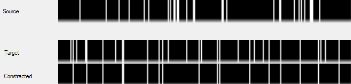
An example of the work of combinatorial space in the learning process (about 200 steps). At the top, the source code, in the middle is the required code, at the bottom, the code predicted by the combinatorial space.

Gradually, the output of the combinatorial space begins to reproduce better and better the required exit code. After several thousand steps of training, the output is reproduced with sufficiently high accuracy (figure below).


An example of a trained combinatorial space. At the top, the source code, in the middle is the required code, at the bottom, the code predicted by the combinatorial space.

To visualize how it all works, I recorded a video with the learning process. In addition, perhaps, my explanations will help to better understand the whole of this kitchen.

Strengthening the rules

To identify more complex patterns, you can use the brake receptors. That is, to introduce patterns that block the operation of some affirmative rules when a certain combination of input bits appears. It looks like the creation of a receptor cluster with inhibitory properties under certain conditions. When such a cluster is triggered, it will not increase, but decrease the point potential.

It is easy to come up with rules for testing inhibitory hypotheses and start consolidating inhibitory receptive clusters.

Since the brake clusters are created at specific points, they do not affect the blocking of the output bit at all, but the blocking of its triggering from the rules detected at this point. You can complicate the connection architecture and introduce brake rules common to a group of points or for all points connected to the output bit. It seems that you can come up with a lot of interesting things, but for now let's focus on the described simple model.

Random forest

The described mechanism allows you to find patterns that are commonly called in Data Mining “if-then” type rules. Accordingly, it is possible to find something in common between our model and all those methods that are traditionally used to solve such problems. Perhaps the closest to us is “random forest” .

This method begins with the idea of "random subspaces". If there are too many variables in the source data and these variables are weak but correlated, then it becomes difficult to isolate individual patterns in the full amount of data. In this case, you can create subspaces in which both the variables used and the training examples will be limited. That is, each subspace will contain only part of the input data, and this data will not be represented by all the variables, but by their random limited set. For some of these subspaces, the chances of finding patterns that are poorly visible in the full amount of data are greatly increased.

Then, in each subspace, a decision tree is trained on a limited set of variables and training examples.. The decision tree is a tree structure (figure below), at the nodes of which the input variables (attributes) are checked. According to the results of testing the conditions in the nodes, the path from the vertex to the terminal node, which is called the leaf of the tree, is determined. In the leaf of the tree is the result, which can be the value of any value or the class number.


An example of a decision-making tree

For decision trees, there are various learning algorithms that allow you to build a tree with more or less optimal attributes in its nodes.

At the final stage, the idea of boosting is applied . Decisive trees form a committee for voting. Based on collective opinion, the most plausible answer is created. The main advantage of boosting is the possibility of combining the set of “bad” algorithms (the result of which is only slightly better than random) to obtain an arbitrarily “good” final result.

In our algorithm, which exploits combinatorial space and receptor clusters, the same fundamental ideas are used as in the random forest method. Therefore, it is not surprising that our algorithm works and gives a good result.

Learning biology

Actually, this article describes the software implementation of the mechanisms that were described in the previous parts of the cycle. Therefore, we will not repeat everything from the very beginning, we only note the main thing. If you forgot about how a neuron works, then you can re-read the second part of the cycle .

On the membrane of the neuron there are many different receptors. Most of these receptors are in "free swimming." The membrane creates an environment for the receptors in which they can move freely, easily changing their position on the surface of the neuron (Sheng, M., Nakagawa, T., 2002) (Tovar KR, Westbrook GL, 2002).


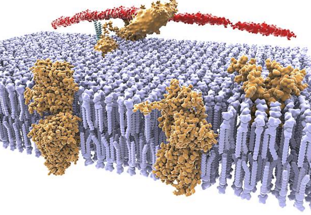
Membrane and receptors

In the classical approach, the reasons for this “freedom” of receptors are usually not emphasized. When a synapse increases its sensitivity, it is accompanied by the movement of receptors from the extra-synaptic space into the synaptic cleft (Malenka RC, Nicoll RA, 1999). This fact is tacitly perceived as an excuse for receptor motility.

In our model, we can assume that the main reason for the mobility of receptors is the need to form clusters of them on the fly. That is, the picture is as follows. A wide variety of receptors sensitive to various neurotransmitters drift freely along the membrane. The information signal that has arisen in the minicarrier causes the release of neurotransmitters by axonal neuron and astrocyte endings. In every synapse where neurotransmitters are emitted, besides the main neurotransmitter, there is a unique additive that identifies this particular synapse. Neurotransmitters spill out of synaptic crevices into the surrounding space, due to which a specific cocktail of neurotransmitters appears in each place of the dendrite (points of the combinatorial space) (the cocktail ingredients indicate bits that hit the spot).Those free-wandering receptors that at this moment find their neurotransmitter in this cocktail (receptors of specific bits of the input signal) are moving into a new state - the search state. In this state, they have a short time (until the next clock cycle occurs), during which they can meet other “active” receptors and create a common cluster (a cluster of receptors that are sensitive to a particular combination of bits).

Metabotropic receptors, and we are talking about them, have a rather complex shape (figure below). They consist of seven transmembrane domains that are connected by loops. In addition, they have two free ends. Due to electrostatic charges of different sign, the free ends can stick to each other through the membrane. Due to such compounds, the receptors and clustered.


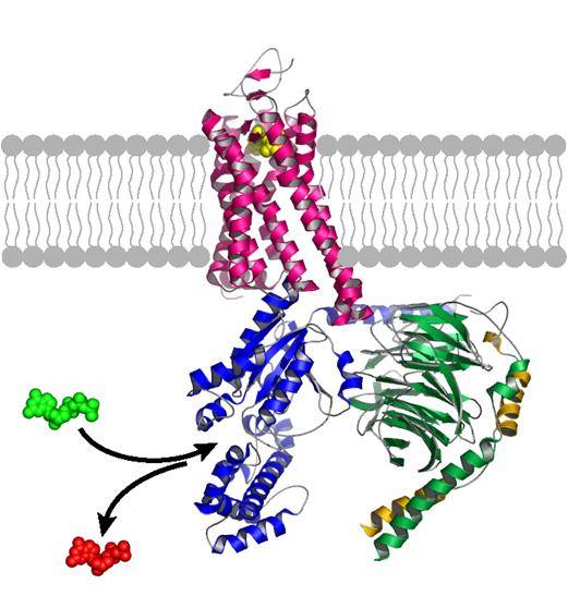
Single metabotropic receptor

After unification, the joint life of the receptors in the cluster begins. It can be assumed that the position of the receptors relative to each other can vary within wide limits and the cluster can take odd forms. If we assume that receptors that work together will tend to take a place closer to each other, for example, due to electrostatic forces, then we get an interesting consequence. The closer such “joint” receptors appear to be, the stronger their joint attraction will be. Having come closer they will begin to strengthen the influence of each other. This behavior reproduces the behavior of the Hebb filter, which selects the first main component. The more precisely the filter is tuned to the main component, the stronger is its reaction when it appears in the example. In this way,if, after a series of iterations, jointly triggered receptors will be together in the conditional “center” of the cluster, and the “extra” receptors at a distance, on its edges, then, in principle, such “extra” receptors may self-destruct at some point, that is, just come off from the cluster. And then we get the behavior of the cluster, similar to that described above in our computational model.

Clusters that have gone through consolidation can move somewhere “to a safe haven”, for example, to the synaptic cleft. There exists a postsynaptic compaction for which clusters of receptors can anchor, losing mobility that they no longer need. There will be ion channels near them that they can control via G-proteins. Now, these receptors will begin to influence the formation of a local postsynaptic potential (potential points).

The local potential is made up of the joint influence of the nearby activating and inhibiting receptors. In our approach, activators are responsible for recognizing patterns that call for activating the output bit, inhibiting the identification of patterns that block the effect of local rules.

Synapses (dots) are located on the dendritic tree. If somewhere on this tree there is a place where several activating receptors are triggered in a small area and this is not blocked by inhibitory receptors, then a dendritic spike occurs, which spreads to the neuron body and, after reaching the axon mound, causes the neuron spike. A dendritic tree combines many synapses, closing them into one neuron, which is very similar to the formation of the output bit of a combinatorial space.

Combining signals from different synapses of a single dendritic tree can be not a simple logical addition, but it can be more difficult and implement some algorithm of clever boosting.

Let me remind you that the basic element of the cortex is a cortical minicolon. In the minicolumn about a hundred neurons are located under each other. At the same time, they are tightly shrouded in bonds, which are much more abundant inside the minicolumn, than the bonds leading to neighboring minicolumns. The entire cortex of the brain is the space of such minicolumns. One neuron of a minicolumn can correspond to one output bit, all neurons of a single cortical minicolumn can be analogous to an output binary vector.

The clusters of receptors described in this chapter create the memory responsible for the search for patterns. We have previously described how to create holographic event memory using receptor clusters. These are two different types of memory that perform different functions, although based on common mechanisms.

Sleep

In a healthy person, sleep begins with the first stage of slow sleep, which lasts 5-10 minutes. Then comes the second stage, which lasts about 20 minutes. Another 30-45 minutes are in the periods of the third and fourth stages. After that, the sleeper returns to the second stage of slow sleep, after which the first episode of REM sleep occurs, which has a short duration of about 5 minutes. During REM sleep, the eyeballs very often and periodically make quick movements under closed eyelids. If at this time to wake the sleeper, then in 90% of cases you can hear the story of a vivid dream. This whole sequence is called a loop. The first cycle has a duration of 90-100 minutes. Then the cycles are repeated, while the proportion of slow sleep decreases and the proportion of REM sleep gradually increases.the last episode of which in some cases can reach 1 hour. On average, with full healthy sleep, there are five complete cycles.

It can be assumed that the main work on clearing clusters of receptors that have accumulated during the day occurs in a dream. In the computational model, we described the procedure of “idle” learning. Old experience is presented to the brain without causing the formation of new clusters. The goal is to test existing hypotheses. This verification consists of two stages. The first is the calculation of the main component of the pattern and the verification that the number of bits responsible for it is sufficient for clear identification. The second is the verification of the truth of the hypothesis, that is, that the pattern is at the right point associated with the desired output bit. It can be assumed that part of the night sleep stages is associated with such procedures.

All processes associated with changes in cells are accompanied by the expression of certain proteins andtranscription factors . There are proteins and factors about which it is shown that they are involved in the formation of a new experience. So, it turns out that their number greatly increases during wakefulness and decreases sharply during sleep.

It is possible to see and estimate the concentration of proteins through staining of a section of brain tissue with a dye that selectively reacts to the desired protein. Similar observations have shown that the most extensive changes in memory proteins are occurring during sleep (Chiara Cirelli, Giulio Tononi, 1998) (Cirelli, 2002) (figures below).


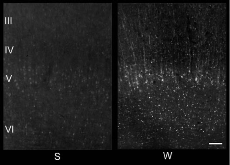
Arc protein distribution in rat parietal cortex after three hours of sleep (S) and after three hours of spontaneous wakefulness (W) (Cirelli, 2002)


Distribution of the P-CREB transcription factor in the coronal areas of the rat parietal cortex after three hours of sleep (S) and in the case of sleep deprivation for three hours (SD) (Cirelli, 2002)

Such a reasoning about the role of sleep fits well with the well-known feature - “the morning of the evening is wiser”. In the morning we are much better oriented in what was not very clear yesterday. Everything becomes clearer and clearer. It is possible that we are obliged by this large-scale clearing of clusters of receptors that occurred during sleep. False and dubious hypotheses are removed, reliable ones are consolidated and begin to actively participate in information processes.

When modeling it was seen that the number of false hypotheses is many thousands of times higher than the number of true ones. Since it is possible to distinguish one from another only by time and experience, the brain has no choice but to save all this information ore in the hope of finding grams of radium in it over time. When new experiences are received, the number of clusters with hypotheses requiring verification is constantly growing. The number of clusters formed per day and containing ore that has yet to be processed may exceed the number of clusters responsible for coding the accumulated experience gained over the entire previous life. The brain's resource for storing raw hypotheses requiring verification should be limited. It seems that in 16 hours of daytime wakefulness, all available space is almost completely clogged with clusters of receptors. When this moment comes, the brain starts forcing us to go to sleep, to allow it to consolidate and clear the free space. Apparently, the process of complete clearance takes about 8 hours. If you wake up earlier, part of the clusters will remain unprocessed. Hence the phenomenon that fatigue accumulates. If you do not have enough sleep for a few days, then you have to catch up with the lost sleep. Otherwise, the brain starts “abnormally” deleting clusters, which does not lead to anything good, since it deprives us of the opportunity to learn from our experience. Event memory is likely to remain, but the patterns will remain undetected.
By the way, my personal advice: do not neglect the quality of sleep, especially if you are learning. Do not try to save on a dream in order to have more time. Sleep is no less important in learning than attending lectures and repeating material in practical classes. No wonder children in those periods of development, when the accumulation and synthesis of information is most active, most of the time is spent in a dream.

Brain speed

The assumption of the role of receptive clusters makes it possible to take a fresh look at the question of the speed of the brain. Earlier we said that each minicolon of the cortex, consisting of hundreds of neurons, is an independent computational module that considers the interpretation of the incoming information in a separate context. This allows one zone of the cortex to consider up to a million possible treatment options at the same time.

Now we can assume that each cluster of receptors can work as an autonomous computing element, performing the entire cycle of calculations to test its hypothesis. There can be hundreds of millions of such clusters in a cortical column alone. This means that, although the frequencies with which the brain works are far from the frequencies at which modern computers work, there is no need to worry about the speed of the brain. Hundreds of millions of clusters of receptors working in parallel in each minicolumn of the cortex, can successfully solve complex problems that are on the border with a combinatorial explosion. Miracles do not happen. But you can learn to walk on the brink.

The text of the given program is available on GitHub . There are quite a few debug fragments left in the code, I didn’t delete them, I just commented out in case anyone wanted to experiment on their own.

Alexey Redozubov

The logic of consciousness. Part 1. Waves in the cellular automaton
The logic of consciousness. Part 2. Dendritic waves
The logic of consciousness. Part 3. Holographic memory in a cellular automaton
The logic of consciousness. Part 4. The secret of brain memory
The logic of consciousness. Part 5. The semantic approach to the analysis of information
The logic of consciousness. Part 6. The cerebral cortex as a space for calculating meanings.
The logic of consciousness. Part 7. Self-organization of the context space
The logic of consciousness. Explanation "on the fingers"
The logic of consciousness. Part 8. Spatial maps of the cerebral cortex
The logic of consciousness. Part 9. Artificial neural networks and minicolumns of the real cortex.
The logic of consciousness. Part 10. The task of generalization
The logic of consciousness. Part 11. Natural coding of visual and sound information
The logic of consciousness. Part 12. The search for patterns. Combinatorial space