Oscillating link model in resonant oscillation mode in Python
Introduction
In article [1], I strictly considered the oscillatory component in strict accordance with the well-known theory of oscillatory processes, constructing transient processes using the SymPy and NumPy libraries.
The first was considered the case of aperiodic and free damped oscillations, initiated by an infinite impulse of constant amplitude force.
The second was a case of negative damping (which I did not comment on). Negative damping can be observed when, under a horizontally suspended center on two springs, the cube is moving a tape swinging with one of its faces.
')
The tape involves the cube in the movement of friction against the surface of the face. When the elastic forces of the springs acting in one direction exceed the friction force, the cube returns to the initial position and the oscillating cycle repeats. As for the oscillatory level, it has been studied sufficiently and has no reason to pretend to scientific research. However, I hope that Python lovers the solution itself was not uninteresting. Now, with the same hope, I want to disassemble a more complex case of the behavior of an oscillatory link under the action of an exciting force changing according to a harmonic law at the resonance frequency of the system.
I will begin with the trivial differential equation of motion, which describes a mechanical oscillatory system with a concentrated mass, stiffness and damping.
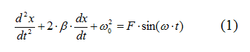
In equation (1) the following notation is used:
F = f / m is the reduced amplitude of the force that oscillates;
 ─ attenuation coefficient;
 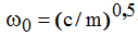 ─ natural frequency of the system;
  ─ frequency of force forcing fluctuations; m ─ concentrated mass; r is the damping coefficient; c ─ concentrated stiffness of the oscillatory system; x is the coordinate of the movement; t is the time coordinate; f is the amplitude of the force oscillating.
Consider the program code for the numerical solution of equation (1)
import numpy as np from sympy import * from IPython.display import * import matplotlib.pyplot as plt import matplotlib as mpl mpl.rcParams['font.family'] = 'fantasy' mpl.rcParams['font.fantasy'] = 'Comic Sans MS, Arial' init_printing(use_latex=True) var('t C1 C2') u = Function("u")(t) B=0.1# w=10# f=1# de = Eq(u.diff(t, t) +2*B*u.diff(t) +w**2* u, f*sin(w*t))# display(de)# IDLE des = dsolve(de,u)# display(des)# IDLE eq1=des.rhs.subs(t,0)# display(eq1)#) 1,2 IDLE eq2=des.rhs.diff(t).subs(t,0)# display(eq2)# 1,2 IDLE seq=solve([eq1,eq2],C1,C2)# 1,2 display(seq)# 1,2 IDLE rez=des.rhs.subs([(C1,seq[C1]),(C2,seq[C2])])# 1,2 display(rez)#) IDLE g= lambdify(t, rez, "numpy")# NumPy t= np.linspace(0,2*w,1000)# 0-2*w 1000 tt=[ i for i in t if g(i)==max(g(t))]# plt.title(' B -%f,'%B)# plt.xlabel(' - %i% tt[0], fontsize=12) plt.ylabel(' -%f'%(2*max(g(t))),fontsize=16) plt.plot(t,g(t),color='b', linewidth=3) plt.grid(True) plt.show() The proposed code is intended to study the resonant when the frequency of the driving force w is equal to the natural frequency w of the mechanical system. For clarity of graphs, the frequency is selected as low w = 10 s-1
Using Python + SymPy + NumPy, unlike publications known to me on the network, allows not only to solve equation (1) but also to establish the amplitude range - max (g (t)), but also to determine the time for establishing self-oscillations - tt = [i for i in t if g (i) == max (g (t))]
The results of solving a differential equation in the given program in Python are comparable to the solution in the ONLINE service [2].
The original equation in Python. Lines of code to output.
de = Eq (u.diff (t, t) + 2 * B * u.diff (t) + w ** 2 * u, f * sin (w * t))
display (de)
Result
: Eq (100 * u (t) + 0.2 * Derivative (u (t), t) + Derivative (u (t), t, t), sin (10 * t))
For service.

Common Python Solution: Eq (u (t), (C1 * sin (3 * sqrt (1111) * t / 10) + C2 * cos (3 * sqrt (1111) * t / 10)) / exp (t) ** (1/10) - 0.5 * cos (10 * t))
General solution on the service:
Constant coefficients C1, C2 in Python
{C2: 0.500000000000000, C1: 0.00500025001875156}
On the service.

The comparison confirms the identity of the developed solution scheme to the service [2] both in terms of the solution and in the result.
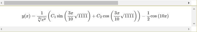
Let's return to the oscillatory link. Set the following attenuation values B = [0.1,0.25,0.5], leaving the remaining parameters of the oscillating system unchanged, we obtain the following graphs.

Stages of solving the differential equation of oscillations.
Eq (100 * u (t) + 0.2 * Derivative (u (t), t) + Derivative (u (t), t, t), sin (10 * t))
Eq (u (t), (C1 * sin (3 * sqrt (1111) * t / 10) + C2 * cos (3 * sqrt (1111) * t / 10)) / exp (t) ** (1 / 10) - 0.5 * cos (10 * t))
C2 - 0.5
3 * sqrt (1111) * C1 / 10 - C2 / 10
{C2: 0.500000000000000, C1: 0.00500025001875156}
(0.00500025001875156 * sin (3 * sqrt (1111) * t / 10) + 0.5 * cos (3 * sqrt (1111) * t / 10)) / exp (t) ** (1/10) - 0.5 * cos ( 10 * t)

Stages of solving the differential equation of oscillations.
Eq (100 * u (t) + 0.5 * Derivative (u (t), t) + Derivative (u (t), t, t), sin (10 * t))
Eq (u (t), (C1 * sin (sqrt (1599) * t / 4) + C2 * cos (sqrt (1599) * t / 4)) / exp (t) ** (1/4) - 0.2 * cos (10 * t))
C2 - 0.2
sqrt (1599) * C1 / 4 - C2 / 4
{C2: 0.200000000000000, C1: 0.00500156323280355}
(0.00500156323280355 * sin (sqrt (1599) * t / 4) + 0.2 * cos (sqrt (1599) * t / 4)) / exp (t) ** (1/4) - 0.2 * cos (10 * t)
Stages of solving the differential equation of oscillations.
Eq (100 * u (t) + 1.0 * Derivative (u (t), t) + Derivative (u (t), t, t), sin (10 * t))
Eq (u (t), (C1 * sin (sqrt (399) * t / 2) + C2 * cos (sqrt (399) * t / 2)) / sqrt (exp (t)) - 0.1 * cos (10 * t))
C2 - 0.1
sqrt (399) * C1 / 2 - C2 / 2
{C1: 0.00500626174321759, C2: 0.100000000000000}
(0.00500626174321759 * sin (sqrt (399) * t / 2) + 0.1 * cos (sqrt (399) * t / 2)) / sqrt (exp (t)) - 0.1 * cos (10 * t)
It follows from the graphs given that the time for establishing resonant oscillations at small dampings does not change significantly (19.8 -19.16. As the attenuation increases, the time change becomes noticeable (19.16-- 17.28). While the amplitude span decreases in proportion to the increase The recovery time of the stationary amplitude of resonant oscillations is an important parameter when using such oscillations, for example, when measuring the added mass.
Conclusion
The proposed model can be used both in the study of resonant processes and for educational purposes.
Links
Source: https://habr.com/ru/post/326296/
All Articles