Neural networks in the fight against cancer

Last year, Arthur Kadurin and I decided to join the new wave of neural network learning - to deep learning. It immediately became clear that machine learning was practically not used in many areas, and we in turn understand how it can be applied. It remained to find an interesting area and strong experts in it. So we met the team from Insilico Medicine (resident of the BMT cluster of the Skolkovo Foundation) and the developers of the MIPT and decided to work together on the task of finding a cure for cancer.

Below you will read a review of the article The cornucopia of meaningful leads: Applying deep adversarial autoencoders for new molecule development in oncology , which my colleagues from Insilico Medicine and MIPT prepared for the American magazine Oncotarget, with an emphasis on the implementation of the proposed model in the tensorflow framework. The initial task was as follows. There are data of a type: substance, concentration, growth rate of cancer cells. It is necessary to generate new substances that would stop the growth of the tumor at a certain concentration. Dataset is available on the NCI Wiki website.

Let's describe the data in more detail.

Substances are presented in the standard for bioinformatics form - SMILES, in fact, it is a unified way to record compounds in ASCII. Unfortunately, there is no complete unification, different packages generate different SMILES. We used those created using the CACTVS package. More about this is written, for example, here . Each SMILES can be converted to a binary representation of the dimension 166: chemical fingerprint, Molecular ACCess System (MACCS). Each bit in this view is the answer to the question about the corresponding molecule, MACCS keys are the set of corresponding questions. Examples of questions: is there less than three oxygen atoms in a molecule? Does the molecule have a ring of size three? A more detailed description is here .

The growth index is defined as follows:

$$

$$GI = \ begin {cases} \ frac {T_i - T_z} {C - T_Z}, & T_i \ ge T_z \\ \ frac {T_i - T_z} {T_z}, & T_i <T_z \ end {cases},$$

Where $$$T_z$- the initial size of the tumor, $$$T_i$- the size of the tumor after a certain time interval in the presence of the drug, $$$C$- tumor size in the control group without the addition of the drug. Actually $$$GI$shows how much slower a tumor grows or how quickly it diminishes.

After the described processing, 78 728 triples of the fingerprint, log (concentration), GI type, describing 6252 molecules, are obtained. To validate the model, we used binary representations for almost 100 million molecules from the Pubchem database ( The PubChem Project ).

An example of the initial data obtained:

Fingerprint	Log (concentration)	Growth inhibition percentage
000011100010 ...	-five	ten %
00000110101 ...	–7	-15 %
10010011000 ...	–4,8	75%

Solutions

Naive approach

The first approach that comes to mind is to train the regressor (for example, xgboost) to determine the growth index by a pair of fingerprint, log (concentration), and then sample such two from a large base and select the best ones.

We could not bring such an approach to anything good.

Generative approach

Another option: learn how to generate pairs (fingerprint, concentration) and then look for similar molecules from a large compound base. One of the first questions: how to compare different molecules? Fortunately (?), We found out experimentally that in this case the Jacquard measure can be used, and for many applications, molecules with a Jacquard coefficient greater than 0.8 are already considered to be close.

In addition to solving the problem as such, we pursued the goal of learning to use new generative neural network approaches. Two modern generative models are known - VAE (variational autoencoder) and GAN (generative adversarial encoder). Since both models have already been described several times on Habré, we confine ourselves to a short story about them.

In the case of VAE , an approximation problem is solved. $$$p (x)$as

$$

$$p (x) = \ int p (x \ mid z; \ theta) p (z) dz,$$

Where $$$x$- input data, $$$z$- latent view, and $$$\ theta$- model parameters.

Standard VAE assumes that $$$p (x \ mid z; \ theta)$and $$$p (z)$normal and brings $$$f (z; \ theta)$using a neural network with an autoencoder structure.

Input data $$$x$served to the input of the encoder, the output of which is a normal distribution $$${\ cal N} (\ mu (x), \ Sigma (x))$. Then the vector is sampled from this distribution. $$$z$which, in turn, is input to the decoder. Outlet - vector $$$y$vector reconstruction $$$x$.

When training a neural network, the average between the two loss functions is optimized: KL divergence between the distribution on the latent layer and $$${\ cal N} (0, I)$and reconstruction error - the distance between $$$x$and $$$y$.

In the case of a GAN, two neural networks are trained: a generator and a discriminator. The generator translates the latent variable $$$z$sampled from prior distribution $$$p (z)$, into the input data space, and the discriminator learns to distinguish the sampled data from the real data. The problem can be formulated in game-theoretic form:

$$

$$\ min_G \ max_D {\ mathbb E} _ {x \ sim p _ {\ mathrm {data}}} [\ log D (x)] + {\ mathbb E} _ {x \ sim p _ {\ mathrm {data} }} [\ log (1 - D (G (z)))]$$

Finally, the Adversarial Autoencoders article introduces a mix of VAE and GAN models. Just like in regular AE, input $$$x$served in the encoder, the output of which $$$z$, in turn, goes to the input to the decoder. The discriminator network learns to distinguish vector $$$e$sampled from $$${\ cal N} (0, I)$and vector $$$z$. As in the GAN, two loss functions are optimized:

• Weights of the generator are optimized to “deceive” the discriminator: not to distinguish $$$e$from $$$z$.
• Discriminator weights are optimized to distinguish $$$e$from $$$z$.

This introduces an additional loss function - reconstruction error. Optimization of loss functions occurs alternately. For example, the first training cycle will look like this: train a discriminator on a mini-batch, train an encoder on the next mini-batch, and train an auto-encoder on a third mini-batch.

The VAE and GAN models have recently become especially popular in image generation tasks, with models based on GAN showing themselves better in practice (for example, NIPS 2016 Tutorial: Generative Adversarial Networks ).

For this reason, and because of the simplicity of adding the growth index to the latent layer of the auto-encoder, we stopped at the last approach to solve a specific problem (we are waiting for the publication of our new article with a detailed comparison of different models). In addition, in the solution of the problem, we could not find the hyperparameters of the standard GAN architecture with which it would work stably.

The model to which we have come is as follows:

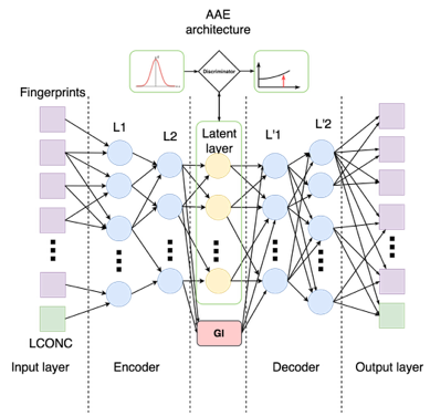
In order for the concentration to influence the output of the encoder as little as possible, we added another loss function - manifold loss:

$$

$$\ sum \ limits_ {1 \ le i <j \ le k} 1 - S_C (E (Fp, C_i), E (Fp, C_j)),$$

Where $$$E$- encoder, and $$$S_c$- cosine measure.

Finally, in the latent layer, we solve the regression problem: from the latent representation of the fingerprint and concentration, determine $$$GI$by adding the corresponding loss function. As a result, each step of training consists of five stages:

1. Learning discriminator weights (as in the GAN).
2. Learning generator weights (as in GAN).
3. Learning autoencoder, i.e. optimization of reconstruction errors.
4. Regressor training.
5. Optimization of the loss function - manifold loss.

The code for the entire learning process is here (at the moment we are continuing to experiment with the code and are going to upload an improved version in the near future).

Let us consider in more detail the implementation of network architecture and metrics. We separate the weights of each part of the network into a separate tf.name_scope in order to be able to optimize them separately. Additionally, we isolate the concentration from the input layer into a separate variable and separately consider the reconstruction error for it.

As usual, the network is a sequence of linear layers and activation functions. For example, the encoder is arranged as follows ( aae_v3.py , lines 109-127):

# Encoder net: 166+1->128->64->3+1 with tf.name_scope("encoder"): encoder = [self.visible_tensor] sizes = [self.input_space + 1, 128, 64, self.latent_space] for layer_number in xrange(encoder_layers): with tf.name_scope("encoder-%s" % layer_number): enc_l = layer_output(sizes[layer_number], sizes[layer_number + 1], encoder[-1], 'enc_l') encoder.append(enc_l) with tf.name_scope("encoder-fp"): self.encoded_fp = layer_output(sizes[-2], sizes[-1], encoder[-1], 'encoded_fp', batch_normed=False, activation_function=identity_function) with tf.name_scope("tgi-encoder"): self.encoded_tgi = layer_output(sizes[-2], 1, encoder[-1], 'encoded_tgi', batch_normed=False, activation_function=identity_function) self.encoded = tf.concat(1, [self.encoded_fp, self.encoded_tgi]) 

Discriminator loss function:

$$

$$\ frac {1} {m} \ sum \ limits_ {i = 1} ^ m \ left [log (Disc (E (x))) + log (1 - Disc (Dec (z)) \ right]$$

To combat overflow, we consider sigmoid not immediately at the discriminator output, but directly inside the loss function. In the code:

 self.disc_loss = tf.reduce_mean(tf.nn.relu(self.disc_prior) - self.disc_prior + tf.log(1.0 +tf.exp(-tf.abs(self.disc_prior)))) + tf.reduce_mean(tf.nn.relu(self.disc_enc) + tf.log(1.0 + tf.exp(-tf.abs(self.disc_enc)))) 

Encoder loss function:

$$

$$\ frac {1} {m} \ sum \ limits_ {i = 1} ^ m \ left [1-log (Disc (E (x))) \ right]$$

In the code:

 self.enc_fp_loss = tf.reduce_mean(tf.nn.relu(self.disc_enc) - self.disc_enc + tf.log(1.0 + tf.exp(-tf.abs(self.disc_enc)))) 

Autoencoder loss function:

$$

$$CrossEntropy (Dec (E (x)), x) + RMSE (Dec (E (c)), c)$$

In the code:

 self.dec_fp_loss = tf.reduce_mean(tf.nn.sigmoid_cross_entropy_with_logits(self.decoded_fp, self.fingerprint_tensor)) self.dec_conc_loss = tf.reduce_mean(tf.square(tf.sub(self.conc_tensor, self.decoded_conc))) self.dec_loss = self.dec_fp_loss + self.dec_conc_loss 

Regressor:

$$

$$RMSE (encoded GI, GI)$$

In the code:

 self.enc_tgi_loss = tf.reduce_mean(tf.square(tf.sub(self.tgi_tensor, self.encoded_tgi))) 

Manifold loss in code:

 fp_norms = tf.sqrt(tf.reduce_sum(tf.square(self.encoded_fp), keep_dims=True, reduction_indices=[1])) normalized_fp = tf.div(self.encoded_fp, fp_norms) cosines_fp = tf.matmul(normalized_fp, tf.transpose(normalized_fp)) self.manifold_cost = tf.reduce_mean(1 - tf.boolean_mask(cosines_fp, self.targets_tensor)) 

In our experiments, the network with different configurations behaved unstably. To increase the stability before the main learning process, we repeated steps 1, 2 and 5 until the discriminator and the encoder reached a state of equilibrium: discriminator_loss <0.7 and encoder_loss <0.7.

Model validation

After training, we generate a random sample of 1000 pairs (fingerprint, concentration) with the condition in a standard way for GAN. $$$GI \ sim 0$:

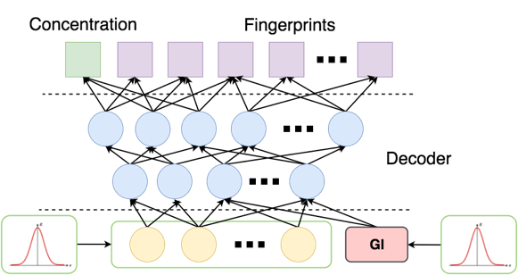
Serve in the latent layer prior distribution, and instead $$$GI$- small numbers with normal noise $$${\ cal N} (5, 1)$(zeros serve badly because the function $$$GI$at this point has a gap). At the output, we obtained 32 probability vectors of fingerprint bits with a concentration of <–5.

Finally, it remains to find real molecules from a large base, similar to the vectors obtained. There are at least three approaches:

• calculate NLL (likelihood log);
• Sample from the obtained distributions as from the multidimensional Bernoulli distributions and calculate the Jaccard distance;
• just put a cutoff of 0.5 and calculate the distance Jacquard.

For each probability vector, we found the top 10 “similar” molecules for each of the three approaches and obtained similar results.

Result

As a result, we found 69 unique substances that were not in the training set. According to data from The PubChem Project , about half of the substances are either already used against cancer, or have a proven effect against cancer. We expect that the remaining half of the substances can also potentially fight cancer.

Thus, a rather naive approach with relatively small input data allowed us to get a good result. It is expected that many problems of bioinformatics can be solved by similar methods.

Unfortunately, in each specific case, the competing networks behave differently and, if the hyper parameters are chosen incorrectly, they converge to the wrong decisions (the generator defeats the discriminator, or vice versa). We are working to find more stable structures and learning methods.