Image filtering by mathematical morphology on FPGA
In this article I want to consider one, in my opinion, noteworthy approach to image filtering by the method of mathematical morphology. Many articles have been written about mathematical morphology, and one of them is located here in Habré. To the reader unfamiliar with this topic, I recommend first reading the material at the link above.
In the article about image filtering, I talked about the filtering method with a median filter. This filter proved to be very good, but it has a number of limitations and inconveniences:
cumbersome even in the implementation of 3x3:
- requires the formation of a window function
- very complicated for expanding the window
- large latency when serially connected with other window functions.
All these inconveniences do not in the least detract from the degree of its applicability in digital image processing systems, however, there is another approach.
Filtration of images using mathematical morphology is a long-known topic, and all I want is to introduce the reader a little closer.
')
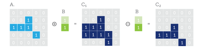
As we have already learned from the article above, from the basic morphological operations narrowing (erosion) and expansion (dilation), we can construct opening (opening) and closing (closing) operations.
The open operation is the sequential execution of erosion -> dilation . This combination will lead to the fact that single pixels and their small clusters will be irretrievably devoured by contraction, as large objects will be gnawed) on the sides. If inside large objects there were small holes, then they will become larger. The subsequent expansion operation will restore the gnawed objects to their original size, but there will no longer be small debris that has been devoured by contraction.
The closing operation is the sequential execution of dilation → erosion . This operation will first fill the holes inside the objects and make them slightly thicker, and then reduce their thickness to the original, but there will be no more holes.
Consecutive opening → closing operations are a very good filter, no worse than the median, but on the contrary, it also makes objects less full of holes. A prerequisite is the same window size for basic operations.
However, each basic erosion or dilation operation is all the same window function, requiring at least 2 FIFOs to implement a 3x3 window and logical AND or OR operations depending on the function.
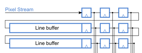
For deeper filtering, a 5x5 and 7x7 window is often used, which entails an increase in the memory capacity of the FIFO elements and the total lag time.
To implement such operations on Altera's FPGAs, you can use the FIFO mega-function and the built-in 2-port memory, but for one such FIFO only 1 bit wide, we don’t need more for a binarized image, such as M4K also not very economical.
Low complexity method
While searching for alternative solutions, I came across the so-called low complexity method on the network. The essence of this method is the decomposition of the matrix of the window function. The initial matrix is decomposed into two:
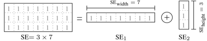
And it works according to this image:
To my shame and regret, I am not strong in mathematics and the topic of decomposition of matrices in the university, I passed, but only by. For this reason, I will not tell you how it works from a mathematical point of view and why it is so and not otherwise for understandable reasons.
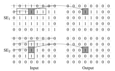
The aforementioned article presented a functional scheme for implementing erosion and dilation operations using the low complexity method. This scheme consists of two blocks, each of which represents a structural element SE1 and SE2 .

From this scheme, it is clear that the choice of erosion / dilation operations is performed by inverting the input data, since these operations are symmetrical.
The output of the Stage-1 block depends on the value of the input pixel and the accumulated sum in the ff trigger. As soon as this sum becomes equal to the width of the window of the structural element SE1, the output of the block will be “1”, otherwise “0”. Any “0” at the block input resets the accumulated amount in the ff trigger to zero. Obviously, this unit counts the number of consecutive units under the structural element SE1 .
The output of the Stage-1 block is fed to the input of the Stage-2 block, which operates on the same principle. The difference from the Stage-1 block is the use of the Row_mem memory depth in the number of columns of the input image, and the amount is stored separately for each column in this memory. The output of the block “1” is only when the sum over the column is equal to the height of the structural element SE2 . The output of the Stage-2 unit can be inverted depending on the erosion or dilation operation performed.
Thus, it turns out that in the Stage-1 block, the circuit tracks all “1” under the horizontal element SE1 and transfers the result to the Stage-2 block, which in turn tracks all the “1” under the vertical element SE2, taking into account the result of the output SE1 .
Also, this scheme provides signals that ensure the operation of the structural element SE at the edges of the image.

The borders of the image are conventionally denoted by the names of the cardinal points: North, South, West and East. When the structural element SE is located at the borders of the image, it is possible to insert ( padding ) the required number of ones or zeros corresponding to the half size of the structural element.
The big advantage of this method is saving memory. The amount of memory required for the Stage-1 and Stage-2 blocks is determined by the word size ( WL ) equal to
Log2 (SE1_width) and Log2 (SE2_height) . For the Stage-2 block, not the trigger is used, but the Row_mem memory, the size of which is Image_width x Log2 (SE2_height) .
Obviously, the result of the calculation of the logarithm must be rounded to the nearest digit capacity SE1_width and SE2_height , i.e. if the window is 3x5, then the rounded value of Log2 (SE1_width) = 2 bits , and Log2 (SE2_height) = 3 bits .
It is not difficult to notice that there is no difference in the use of memory for the 3x3 window in the low complexity method and the usual window method. That in the first case, the amount of memory is 320 columns x 2 bits, which is second: two single-bit FIFO elements of 320 elements each. If the window size changes to 5x5 or 7x7, then the number of FIFOs increases in proportion to the number of rows in the window, but for the low complexity method, the word size will increase by only 1 bit, and the Row_mem memory will be 320x2, not 320x3.
Thus, you can pre-set the maximum window size and use, for example, the altsyncram mega-function of this size. It will be much more economical than using FIFO to form a window function.
The code for the erosion / dilation module in Verilog:
Low complexity erosion / dilation
module low_complexity #(parameter BW = 3'd3, parameter BH = 3'd3, parameter WIDTH = 9'd320, parameter HEIGH = 9'd240, parameter START_X = 9'd320, parameter START_Y = 9'h0 ) ( input wire clk, input wire er_dil, input wire [0:0] data_in, input wire input_valid, input wire [10:0] x_in, y_in, output wire output_valid, output wire [0:0] data_out ); localparam END_X = (WIDTH + START_X) - 1; localparam END_Y = HEIGH - 1; wire e_bound, s_bound, n_bound, w_bound; assign n_bound = (y_in == START_Y && x_in == START_X) ? 1'b1 : 1'b0; assign s_bound = (y_in == END_Y && x_in == END_X) ? 1'b1 : 1'b0; assign w_bound = (x_in == START_X) ? 1'b1 : 1'b0; assign e_bound = (x_in == END_X) ? 1'b1 : 1'b0; // stage 1 wire mux1_out, mux2_out; wire [2:0] mux3_out; wire [2:0] mux4_out; reg [2:0] ff = 0; reg [2:0] ff_d = 0; wire [2:0] sum1; wire [2:0] mux5_out; wire cmp1_out; wire [8:0] mem_addr = input_valid ? x_in[8:0] - START_X : 9'd0; assign mux1_out = er_dil ? ~data_in : data_in; assign mux2_out = (e_bound | s_bound) ? 1'b1 : mux1_out; assign mux3_out = mux2_out ? sum1 : 3'h0; assign mux4_out = cmp1_out ? mux5_out : mux3_out; always @(posedge clk) ff_d = mux4_out; always @* ff = ff_d; assign mux5_out = w_bound ? BH - 1'b1 : ff; assign sum1 = mux5_out + 1'b1; assign cmp1_out = (mux3_out == BW) ? 1'b1 : 1'b0; // stage2 2 wire [2:0] sum2; wire [2:0] mux6_out, mux7_out; wire cmp2_out; wire [2:0] mux8_out; wire [2:0] mem_out; alt_ram320x3 row_mem ( .clock(clk), .data(mux7_out), .rdaddress(mem_addr), .wraddress(mem_addr), .wren(1'b1), .q(mem_out) ); assign mux6_out = cmp1_out ? sum2 : 3'h0; assign mux7_out = cmp2_out ? mux8_out : mux6_out; assign mux8_out = n_bound ? BW : mem_out; assign sum2 = mux8_out + 1'b1; assign cmp2_out = (mux6_out == BH) ? 1'b1 : 1'b0; assign data_out = er_dil ? ~cmp2_out : cmp2_out; assign output_valid = input_valid; endmodule Opening and closing operations:
opening / closing
wire [0:0] er1_out, dil1_out, er2_out, dil2_out; wire dil_input = line_data_out; // OPENING // EROSION 3x3 low_complexity #( .BW(3'h3), .BH(3'h3), .WIDTH(9'd320), .HEIGH(9'd240), .START_X(9'd320), .START_Y(9'h0) ) er_1 ( .clk(clk), .er_dil(1'b0), .data_in(dil_input), .input_valid(line_rd_rq), .x_in(x_in), .y_in(y_in), .output_valid(), .data_out(er1_out) ); // DILATION 3x3 low_complexity #( .BW(3'h3), .BH(3'h3), .WIDTH(9'd320), .HEIGH(9'd240), .START_X(9'd320), .START_Y(9'h0) ) dil_1 ( .clk(clk), .er_dil(1'b1), .data_in(er1_out), .input_valid(line_rd_rq), .x_in(x_in), .y_in(y_in), .output_valid(), .data_out(dil1_out) ); // CLOSING // DILATION 3x3 low_complexity #( .BW(3'h3), .BH(3'h3), .WIDTH(9'd320), .HEIGH(9'd240), .START_X(9'd320), .START_Y(9'h0) ) dil_2 ( .clk(clk), .er_dil(1'b1), .data_in(dil1_out), .input_valid(line_rd_rq), .x_in(x_in), .y_in(y_in), .output_valid(), .data_out(dil2_out) ); // EROSION 3x3 low_complexity #( .BW(3'h3), .BH(3'h3), .WIDTH(9'd320), .HEIGH(9'd240), .START_X(9'd320), .START_Y(9'h0) ) er_2 ( .clk(clk), .er_dil(1'b0), .data_in(dil2_out), .input_valid(line_rd_rq), .x_in(x_in), .y_in(y_in), .output_valid(), .data_out(er2_out) ); Result
This video demonstrates the efficiency of image filtering using the mathematical morphology (low complexity method) with a 3x3 window compared to a median filter with a window of the same size.
Green marker - median filter
Yellow marker - morphology
It is noticeable that unfiltered garbage appears on the video with a green marker and the detector places it in a frame, and in the video with a yellow marker, the garbage disappears and only a large object falls into the frame.
From this experiment, we can conclude that the filter based on mathematical morphology does a little better than the median.
findings
Based on the method of low complexity erosion / dilation, it is possible to construct the basic elements of morphological image processing much more efficiently in terms of memory consumption than by forming a window function.
The result of image filtering by the method of mathematical morphology is no worse than the result of filtering by the median filter, and is a good alternative to the latter.
Materials on the topic
→ Low complexity method
→ Morphological image processing
→ Mathematical morphology
Source: https://habr.com/ru/post/325808/
All Articles