Kinetics of large clusters

Summary

Fatal error Martin Kleppman.
Physico-chemical kinetics do math.
Cluster half-life.
We solve nonlinear differential equations without solving them.
Noda as a catalyst.
Predictive power of graphs.
100 million years.
Synergy.

In the previous article we discussed in detail the article of Brewer and his theorem of the same name . This time we are going to prepare the post of Martin Kleppman, "The probability of data loss in large clusters" .

In this post, the author tries to model the following problem. To ensure data integrity, data replication is usually used. In this case, in fact, it does not matter whether erasure encoding is used or not. In the original post, the author sets the probability of a single node falling out, and then asks: what is the probability of data falling out as the number of nodes increases?

The answer is shown in this picture:

Data loss

')
Those. with the growth of the number of nodes, the number of lost data grows in direct proportion.

Why is it important? If we consider the size of modern clusters, we will see that their number is continuously increasing over time. This means that a reasonable question arises: is it worth worrying about the safety of your data and raising the replication factor? After all, this directly affects the business, cost of ownership and so on. Also using this example, it is possible to demonstrate perfectly how to produce a mathematically correct, but incorrect result.

Cluster modeling

To demonstrate the erroneous calculations it is useful to understand what a model and modeling are. If the model poorly describes the actual behavior of the system, then whatever correct formulas are used, we can easily get the wrong result. And all due to the fact that our model can not take into account some important parameters of the system, which can not be neglected. The art is to understand what is important and what is not.

To describe the life of the cluster, it is important to take into account the dynamics of changes and the interrelation of various processes. This is precisely the weak link of the original article, since there was taken a static picture without any features associated with replication.

To describe the dynamics, I will use the methods of chemical kinetics , where I will use an ensemble of nodes instead of an ensemble of particles. As far as I know, no one used this formalism to describe the behavior of clusters. So I will improvise.

We introduce the following notation:

: total number of nodes in the cluster
: number of functioning nodes (available)
: number of problem nodes (failed)

Then it is obvious that:

$\ begin {aligned} N = A + F \\ \ end {aligned}$

Among the problematic nodes, I will include any problems: the disk is screwed up, the processor, network, etc. broke. The cause is not important to me, the fact of breakdown and unavailability of data is important. In the future, of course, you can take into account the more subtle dynamics.

Now we write the kinetic equations of the processes of breakdown and restoration of the nodes of the cluster:

$\ begin {aligned} A & amp; \ xrightarrow {k_f} F & amp; (1) \\ F & amp; \ xrightarrow {k_a} A & amp; (2) \\ \ end {aligned}$

These simple equations say the following. The first equation describes the process of node failure. It does not depend on any parameters and describes the isolated output of the node down. Other nodes are not involved in this process. On the left is used the original "composition" of participants in the process, and on the right - the products of the process. Speed constants k_f

and

set the speed characteristics of the processes for breaking and restoring the nodes, respectively.

Find out the physical meaning of the rate constants. To do this, we write the kinetic equations:

$\ begin {aligned} \ frac {dA} {dt} & amp; = -k_f A + k_a F \\ \ frac {dF} {dt} & amp; = k_f A - k_a F \\ \ end {aligned}$

From these equations, the meaning of the constants is clear. k_f

and

. Assuming that there are no admins and the cluster does not heal itself (i.e. k_a = 0

), then we immediately get the equation:

$\ begin {aligned} \ frac {dA} {dt} = -k_f A \\ \ end {aligned}$

$\ begin {aligned} A = N e ^ {- k_f t} \\ \ end {aligned}$

Those. magnitude 1 / k_f

Is the half-life of the cluster for parts, up to e / 2

. Let be $\ tau_f$ - the characteristic time of transition of a single node from the state

in state

, but $\ tau_a$ - the characteristic time of transition of a single node from the state

in state

. Then

$\ begin {aligned} \ tau_f & amp; \ sim \ frac {1} {k_f} \\ \ tau_a & amp; \ sim \ frac {1} {k_a} \\ \ frac {\ tau_a} {\ tau_f} & amp; = \ frac {k_f} {k_a} \\ \ end {aligned}$

Solve our kinetic equations. I just want to make a reservation that I will cut corners wherever it is possible, in order to get the simplest possible analytical dependencies that I will use for possible predictions and tuning.

Since the maximum limit on the number of solutions of differential equations has been reached, then I will solve these equations by the method of quasistationary states :

$\ begin {aligned} \ frac {dA} {dt} = 0 \ Rightarrow F = A \ frac {k_f} {k_a} \\ \ end {aligned}$

Given that $F \ ll N$ (this is quite a reasonable assumption, otherwise you need to buy better hardware or more advanced admins), we get:

$\ begin {aligned} A & amp; \ simeq N \\ F & amp; = N \ frac {k_f} {k_a} \\ \ end {aligned}$

If we assume that the recovery time $\ tau_a$ about 1 week and the time of death $\ tau_f$ about 1 year, we find that the proportion of broken nodes p_f

$\ begin {aligned} p_f = \ frac {F} {N} = \ frac {\ tau_a} {\ tau_f} \ approx 2 \% \\ end {aligned}$

Chunky

Denote by

- the number of underreplicated chunks that need to be replicated after the node drops out when going into the state

. Then to account for the chunks, we correct our equations:

$\ begin {aligned} A & amp; \ xrightarrow {k_f} F + U & amp; (1) \\ F & amp; \ xrightarrow {k_a} A & amp; (2) \\ U + A & amp; \ xrightarrow {k_r} H + A & amp; (3) \\ \ end {aligned}$

Where

- the rate constant of replication of the process of the second order, and

means a healthy chunk, which will dissolve in the total mass of chunks.

The 3rd equation needs to be clarified. It describes the second order process, not the first:

$\ begin {aligned} U & amp; \ xrightarrow {k_r} H \\ \ end {aligned}$

If we did that, we would get a Kleppman curve that is not in my plans. In fact, all nodes are involved in the recovery process, and the more nodes, the faster the process goes. This is due to the fact that chunks from a killed node are distributed approximately evenly throughout the cluster, therefore each participant must be replicated in

less time. This means that the final rate of recovery of chunks from a killed node will be proportional to the number of available nodes.

It is also worth noting that in equation (3) on the left and on the right is

, and while it is not consumed. Chemists would immediately say that in this case

acts as a catalyst. And if you think carefully, then it really is.

Using the method of quasistationary concentrations instantly we get the result:

$\ begin {aligned} \ frac {dU} {dt} = 0 = k_f A - k_r U A \\ \ end {aligned}$

$\ begin {aligned} U = \ frac {k_f} {k_r} \\ \ end {aligned}$

Amazing result! Those. the number of chunks that need to be replicated does not depend on the number of nodes! And this is due to the fact that increasing the number of nodes increases the resulting reaction rate (3), thereby compensating for a greater number

nod. Catalysis!

We estimate this value. $\ tau_r$ - recovery time chunks, as if we had only one node. Let 5TB of data be replicated at the node, with the replication stream in bytes set as 50MB / s, then we get:

$\ begin {aligned} U = \ frac {\ tau_r} {\ tau_f} \ approx \ frac {1 \ times 10 ^ 5} {3.2 \ times 10 ^ 7} \ approx 3 \ times 10 ^ {- 3} \\ \ end {aligned}$

Those. $U \ ll 1$ and you can not be afraid for the safety of data. Here it is worth considering that the loss of one chunk out of 3 does not lead to data loss.

Replication planning

In the previous calculation, we made an implicit assumption that the nodes instantly know which chunks need to be replicated, and immediately begin the process of their replication. In reality, this is absolutely not true: the master needs to understand that the node has died, then understand what specific chunks need to be replicated and start the replication process on the nodes. All this is not instantaneous and takes some time. $\ tau_s$ (scheduling).

To account for the delay, we use the theory of a transition state or an activated complex , which describes the process of transition through a saddle point on a multidimensional surface of potential energy. From our point of view, we will have some additional intermediate state U ^ *

which means that this chunk has been scheduled for replication, but the replication process has not yet begun. Those. the next nanosecond replication will begin exactly, but not picosecond earlier. Then our system will take the final form:

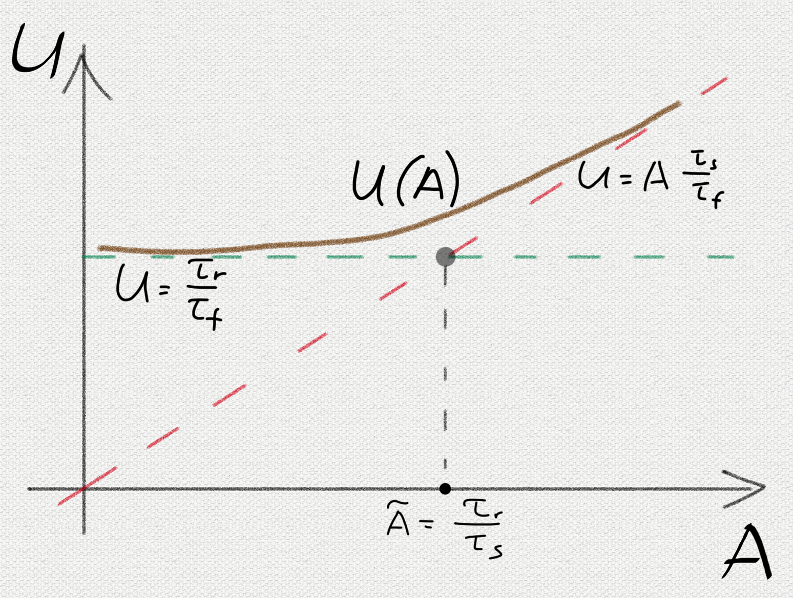
$\ begin {aligned} A & amp; \ xrightarrow {k_f} F + U & amp; (1) \\ F & amp; \ xrightarrow {k_a} A & amp; (2) \\ U & amp; \ xrightarrow {k_s} U ^ * & amp; (3) \\ U ^ * + A & amp; \ xrightarrow {k_r} H + A & amp; (4) \\ \ end {aligned}$

Solving it, we find that:

$\ begin {aligned} \ frac {dU} {dt} & amp; = k_f A - k_s U \\ \ frac {dU ^ *} {dt} & = k_s U - k_r U ^ * A \\ \ end {aligned }$

Using the method of quasistationary concentrations, we find:

$\ begin {aligned} U & amp; = A \ frac {k_f} {k_s} \\ U ^ * & amp; = \ frac {k_f} {k_r} \\ U_ {sum} & amp; = U + U ^ * = \ frac {\ tau_r} {\ tau_f} \ bigg (1 + \ frac {A} {\ widetilde {A}} \ bigg) \\ \ end {aligned}$

Where:

$\ begin {aligned} \ widetilde {A} = \ frac {\ tau_r} {\ tau_s} \\ \ end {aligned}$

As you can see, the result is the same as the previous one, except for the multiplier. $(1 + A / \ widetilde {A})$ . Consider 2 extreme cases:

$A \ ll \ widetilde {A}$ . In this case, all the arguments cited earlier are preserved: the number of chunks does not depend on the number of nodes, and therefore does not grow with the growth of the cluster.
$A \ gg \ widetilde {A}$ . In this case $U_ {sum} \ simeq A \ tau_s / \ tau_f$ and grows linearly with the number of nodes.

To determine the mode, we estimate what is $\ widetilde {A}$ . $\ tau_s$ - this is the characteristic total time of detecting an underreplicated chunk and planning its replication. A rough estimate (using the “finger to the sky” method) gives a value of 100 s. Then:

$\ begin {aligned} \ widetilde {A} = \ frac {1 \ times 10 ^ 5} {100} = 1000 \\ \ end {aligned}$

Thus, a further increase in the cluster above this figure under these conditions will begin to increase the probability of losing chunk.

What can be done to improve the situation? It would seem that the asymptotics can be improved by shifting the border. $\ widetilde {A}$ by increasing $\ tau_r$ however this will only increase the value $U_ {sum}$ without any real improvement. The surest way: this reduction $\ tau_s$ i.e. decision time for chunk replication, since $\ tau_f$ depends on the characteristics of the hardware and this is hard to influence with software.

Discussion of marginal cases

The proposed model actually breaks the aggregate clusters into 2 camps.

A relatively small cluster with the number of nodes <1000 adjoins the first camp. In this case, the probability of obtaining an under-replicated chunk is described by a simple formula:

$\ begin {aligned} U = \ frac {\ tau_r} {\ tau_f} \\ \ end {aligned}$

To improve the situation, you can use 2 approaches:

Improve iron, thereby increasing $\ tau_f$ .
Accelerate replication by reducing $\ tau_r$ .

These methods are generally fairly obvious.

In the second camp, we have already large and super-large servers with the number of nodes> 1000. Here the dependence will be determined as follows:

$\ begin {aligned} U = A \ frac {\ tau_s} {\ tau_f} \\ \ end {aligned}$

Those. will be directly proportional to the number of nodes, which means a subsequent increase in the cluster will adversely affect the likelihood of under-replicated chunks. However, here you can significantly reduce the negative effects using the following approaches:

Continue to increase $\ tau_f$ .
Accelerate the detection of under-replicated chunks and subsequent replication planning, thereby reducing $\ tau_s$ .

2nd reduction approach $\ tau_s$ is no longer obvious. It would seem, what's the difference, will take 20 seconds or 100 seconds? However, this value significantly affects the probability of under-replicated chunks. Also unclear is the fact that the dependence on $\ tau_r$ i.e. the replication speed itself does not matter. It is understandable in this model: with an increase in the number of nodes, this speed only increases, therefore, the constant addition of the “acceleration” of the replication process, aimed at detecting and scheduling replication, begins to significantly affect the chunk replication.

Worth a little more detail on $\ tau_f$ . In addition to directly contributing to the livelihoods of chunks, $\ tau_f$ It has a beneficial effect on the number of available nodes, since

$\ begin {aligned} A = N - F \ simeq N \ bigg (1 - \ frac {\ tau_a} {\ tau_f} \ bigg) \\ \ end {aligned}$

Thereby increasing the number of available nodes. Thus, the improvement $\ tau_f$ directly affects the availability of available cluster resources, speeding up calculations and at the same time increasing the reliability of data storage. On the other hand, improving the quality of iron directly affects the cost of ownership of the cluster. The described model allows us to quantify the economic feasibility of such decisions.

Comparison of approaches

In conclusion, I would like to give a comparison of the two approaches. About this eloquently say the following graphics.

Data loss

From the first graph, you can only see a linear relationship, but it will not give an answer to the question: “and what needs to be done to improve the situation?” The second picture describes a more complex model that can immediately answer questions about what to do and how affect the behavior of the replication process. Moreover, it gives a recipe for a quick way, literally in the mind, of evaluating the consequences of certain architectural decisions. In other words, the predictive power of the developed model is at a qualitatively different level.

Loss of chunk

We now find the characteristic time of chunk loss. To do this, write down the kinetics of the formation of such chunks, taking into account the degree of replication = 3:

$\ begin {aligned} A & amp; \ xrightarrow {k_f} F + U \\ F & amp; \ xrightarrow {k_a} A \\ U & amp; \ xrightarrow {k_s} U ^ * \\ U ^ * + A & amp; \ xrightarrow {k_r} H + A \\ U & amp; \ xrightarrow {k_f} F + U_2 \\ U ^ * & amp; \ xrightarrow {k_f} F + U_2 \\ U_2 & amp; \ xrightarrow {k_s} U_2 ^ * \\ U_2 ^ * + A & amp; \ xrightarrow {k_r} U + A \\ U_2 & amp; \ xrightarrow {k_f} F + L \\ U_2 ^ * & amp; \ xrightarrow {k_f} F + L \\ \ end {aligned}$

Here through U_2

indicated the number of under-replicated chunks that are missing two copies, U_2 ^ *

- intermediate state, similarly U ^ *

corresponding to the state U_2

, but

means a lost chunk. Then:

$\ begin {aligned} \ frac {dL} {dt} & amp; = k_f \ big (U_2 + U_2 ^ * \ big) \\ \ tau_l & amp; = \ frac {1} {k_f \ big (U_2 + U_2 ^ * \ big)} \\ \ end {aligned}$

Where $\ tau_l$ - the characteristic time of formation of the lost chunk. We will solve our system for 2 extreme cases for the case when A = 1000

.

$A \ ll \ widetilde {A}$ then

$\ begin {aligned} \ tau_l = A \ frac {\ tau_f ^ 3} {\ tau_r ^ 2} \ approx 100 \ 000 \ 000 \ years \\ \ end {aligned}$

For $A \ gg \ widetilde {A}$ we get:

$\ begin {aligned} \ tau_l = \ frac {\ tau_f ^ 3} {A \ tau_s ^ 2} \ approx 100 \ 000 \ 000 \ years \\ \ end {aligned}$

Those. the characteristic time of formation of a lost chunk is 100 million years! At the same time, approximately similar values are obtained, since we are in a transition zone. Characteristic time $\ tau_l$ speaks for itself and everyone can draw conclusions himself.

It is, however, worth paying attention to one feature. In the limiting case $A \ ll \ widetilde {A}$ while

is constant and does not depend on

in terms of $\ tau_l$ we get the inverse relationship, i.e. With cluster growth, triple replication even improves data integrity! With further cluster growth, the situation changes exactly to the opposite.

findings

The article consistently introduces an innovative way of modeling the kinetics of large cluster processes. The considered approximate model of cluster dynamics description allows calculating probabilistic characteristics describing data loss.

Of course, this model is only the first approximation to what is really happening on the cluster. Here we only took into account the most significant processes for obtaining a qualitative result. But even such a model makes it possible to judge what is happening inside the cluster, and also gives recommendations for improving the situation.

Nevertheless, the proposed approach allows for more accurate and reliable results based on the subtle consideration of various factors and the analysis of real data on the work of the cluster. The following is far from an exhaustive list for improving the model:

Cluster nodes can fail due to various hardware failures. The failure of a particular node usually has a different probability. Moreover, a failure, for example, of a processor, does not lose data, but only gives temporary unavailability of the node. It is easy to take into account in the model, introducing various states. $F_ {proc}$ , $F_ {disk}$ , $F_ {mem}$ etc. with different speeds of processes and various consequences.
Not all nodes are equally useful. Different batches may differ in character and frequency of failures. This can be taken into account in the model by entering , etc. with different speeds of the respective processes.
Adding various types of nodes to the model: with partially damaged disks, banned, etc. For example, you can analyze in detail the effect of turning off an entire rack and determining the characteristic speeds of a cluster transition to a stationary mode. In this case, numerically solving the differential equations of processes, we can visually consider the dynamics of chunks and nodes.
Each disk has slightly different read / write characteristics, including latency and throughput. Nevertheless, it is possible to more accurately estimate the rate constants of the processes, integrating over the corresponding distribution functions of the characteristics of the disks, by analogy with the rate constants in gases, integrated over the Maxwell distribution of speeds .

Thus, the kinetic approach allows, on the one hand, to obtain a simple description and analytical dependencies, on the other hand, it has a very serious potential for introducing additional subtle factors and processes based on the analysis of cluster data, adding specific points as needed. It is possible to evaluate the impact of the contribution of each factor on the resulting equations, allowing you to simulate the improvements with a view to their expediency. In the simplest case, such a model allows you to quickly obtain analytical dependencies, giving recipes for improving the situation. In this case, the simulation can be bidirectional: you can iteratively improve the model by adding processes to the system of kinetic equations; so try to analyze potential system improvements by introducing relevant processes into the model. Those. to carry out modeling of improvements to the direct costly implementation of them in the code.

In addition, one can always proceed to the numerical integration of a system of rigid nonlinear differential equations, obtaining the dynamics and response of the system to specific actions or small perturbations.

Thus, the synergy of seemingly unrelated areas of knowledge allows you to get amazing results that have undeniable predictive power.

Grigory Demchenko, developer of YT

Literature

[1] Cap Theorem Myths
[2] Spanner, TrueTime and the CAP Theorem
[3] The number of data loss in large clusters
[4] Chemical Kinetics
[5] The activated complex theory
[6] Approximate methods of chemical kinetics
[7] Maxwell distribution
[8] YT: Why does Yandex need its own MapReduce-system and how it works?

Source: https://habr.com/ru/post/325798/

All Articles