Oscillating link model using symbolic and numerical solutions of a differential equation on SymPy and NumPy
Task
This article uses the capabilities of the SymPy package in conjunction with the NumPy package. It all comes down to converting symbolic expressions into functions that can work with other Python modules.
The process of solving differential equations becomes visual and well controlled at each stage of computation. It should be noted that the oscillatory link in different interpretations is discussed in networks [1,2]. For example, in [3], a model of an oscillatory link with a detailed study of transients is presented.
I hope that similar studies of the vibrational link in Python will find their supporters.
')
Program code
In order not to bore the reader, I will cite immediately the program code with an explanation of each significant line.
Code
import numpy as np from sympy import * from IPython.display import * import matplotlib.pyplot as plt init_printing(use_latex=True) var('t C1 C2') u = Function("u")(t) # , . m=20 # . w=10.0# . c=0.3# . a=1# . # ( ). t# . de = Eq(m*u.diff(t,t)+w*u.diff(t)+c*u,a) #- . display(de)#- . des = dsolve(de,u)# . display(des)# . eq1=des.rhs.subs(t,0);# t=0. display(eq1)# . eq2=des.rhs.diff(t).subs(t,0)# # t=0. display(eq2)# . seq=solve([eq1,eq2],C1,C2)# C1,C2. display(seq)# . rez=des.rhs.subs([(C1,seq[C1]),(C2,seq[C2])])# # . display(rez)# . f=lambdify(t, rez, "numpy")# # numpy . x = np.arange(0.0,500,0.01) plt.plot(x,f(x),color='b', linewidth=3) plt.xlabel('Time t seconds',fontsize=12) plt.ylabel('$f(t)$',fontsize=16) plt.grid(True) plt.show() We adjust the damping and obtain an aperiodic motion and all stages of solving the equation.

Eq (0.3 * u (t) + 10.0 * Derivative (u (t), t) + 20 * Derivative (u (t), t, t), 1)
Eq (u (t), C1 * exp (t * (- 5 - sqrt (19)) / 20) + C2 * exp (t * (- 5 + sqrt (19)) / 20) + 3.33333333333333)
C1 + C2 + 3.33333333333333
C1 * (- 1/4 - sqrt (19) / 20) + C2 * (- 1/4 + sqrt (19) / 20)
{C1: 0.245131115588015, C2: -3.57846444892135}
0.245131115588015 * exp (t * (- 5 - sqrt (19)) / 20) - 3.57846444892135 * exp (t * (- 5 + sqrt (19)) / 20) + 3.33333333333333
Let's change the parameters and rewrite the program listing to display three movements with increasing damping on one graph.
Program code for three different values of the damping index
import numpy as np from sympy import * from IPython.display import * import matplotlib.pyplot as plt init_printing(use_latex=True) var('t C1 C2') u = Function("u")(t) # , . m=200 # . w=1.8# . c=1.3# . a=1# . # ( ). t# . man=[0.8,2.12,5]# ( ). for w in man: de = Eq(m*u.diff(t,t)+w*u.diff(t)+c*u,a) #- . display(de)#- . des = dsolve(de,u)# . display(des)# . eq1=des.rhs.subs(t,0);# t=0. display(eq1)# . eq2=des.rhs.diff(t).subs(t,0)# t=0. display(eq2)# . seq=solve([eq1,eq2],C1,C2)# C1,C2. display(seq)# . rez=des.rhs.subs([(C1,seq[C1]),(C2,seq[C2])])# # . display(rez)# . f=lambdify(t, rez, "numpy")# numpy . x = np.arange(0.0,500,0.01) if w==man[0]:# . plt.plot(x,f(x),color='r', linewidth=3) elif w==man[1]: plt.plot(x,f(x),color='g', linewidth=3) elif w==man[2]: plt.plot(x,f(x),color='b', linewidth=3) plt.xlabel('Time t seconds',fontsize=12) plt.ylabel('$f(t)$',fontsize=16) plt.grid(True) plt.show() Set the value of the damping parameter and get a graph of the periodic damped motion and all the stages of solving three equations.
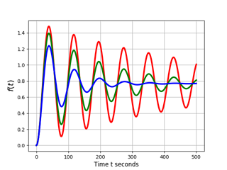
Eq (1.3 * u (t) + 0.8 * Derivative (u (t), t) + 200 * Derivative (u (t), t, t), 1)
Eq (u (t), (C1 * sin (sqrt (406) * t / 250) + C2 * cos (sqrt (406) * t / 250)) / exp (t) ** (1/500) + 0.769230769230769 )
C2 + 0.769230769230769
sqrt (406) * C1 / 250 - C2 / 500
{C2: -0.769230769230769, C1: -0.0190881410379025}
(-0.0190881410379025 * sin (sqrt (406) * t / 250) - 0.769230769230769 * cos (sqrt (406) * t / 250)) / exp (t) ** (1/500) + 0.769230769230769
Eq (1.3 * u (t) + 2.12 * Derivative (u (t), t) + 200 * Derivative (u (t), t, t), 1)
Eq (u (t), (C1 * sin (sqrt (647191) * t / 10000) + C2 * cos (sqrt (647191) * t / 10000)) / exp (t) ** (53/10000) + 0.769230769230769 )
C2 + 0.769230769230769
sqrt (647191) * C1 / 10000 - 53 * C2 / 10000
{C2: -0.769230769230769, C1: -0.0506776284001243}
(-0.0506776284001243 * sin (sqrt (647191) * t / 10000) - 0.769230769230769 * cos (sqrt (647191) * t / 10000)) / exp (t) ** (53/10000) + 0.769230769230769
Eq (1.3 * u (t) + 5 * Derivative (u (t), t) + 200 * Derivative (u (t), t, t), 1)
Eq (u (t), (C1 * sin (sqrt (1015) * t / 400) + C2 * cos (sqrt (1015) * t / 400)) / exp (t) ** (1/80) + 0.769230769230769 )
C2 + 0.769230769230769
sqrt (1015) * C1 / 400 - C2 / 80
{C2: -0.769230769230769, C1: -0.120724003956605}
(-0.120724003956605 * sin (sqrt (1015) * t / 400) - 0.769230769230769 * cos (sqrt (1015) * t / 400)) / exp (t) ** (1/80) + 0.769230769230769
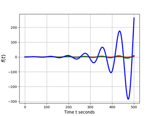
Reduce the mass index and get the motion graphics (the solution of the equations for the reduction is missing).

Let us consider the important case of negative damping and obtain the corresponding graph (the solution of the equations for reduction is missing).
Conclusion
The resulting graphic illustration of the work of an oscillatory link is fully consistent with the theory.
Symbolic and numerical solutions of the differential equation on SymPy and NumPy allowed us to create an adequate model of the oscillatory component with mass control damping and stiffness while controlling the progress of the oscillation equation. In addition, Python is conditionally free software, which greatly expands the possibilities of using the given program for research and educational purposes.
Links
Source: https://habr.com/ru/post/325650/
All Articles