R, GIS and fuzzyjoin: restore statistics for the NUTS regions

In this post we will talk about how I restored the demographic data for the regions of Denmark, where after the reform of the territorial structure of 2007 there was no official data harmonization. This is only a small part of the harmonization of Eurostat data, which I performed as part of my phd project . The post was first published in my English-language blog and Demotrends blog. I think that it may be of some interest not only to demographers.

What is NUTS?

NUTS stands for Nomenclature of Territorial Units For Statistics . This is a standardized system of administrative and territorial division adopted by the EU countries. The story goes back to the 1970s, when the idea was born to make the regions of various European countries comparable. In a more or less complete and widely used form, the system appeared only at the turn of the century. There are three main levels of NUTS (see Fig. 1), and NUTS-2 is the most common in regional analysis.

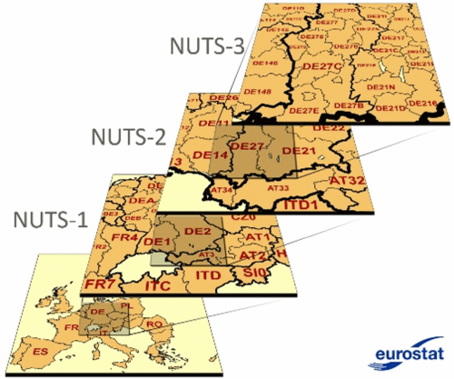
Figure 1. Illustration of the principle of distinguishing NUTS regions of various hierarchical levels

The main task of NUTS was to create comparable criteria for identifying regions of different hierarchical levels. However, in 2013, the population of the Regins of the NUTS-2 level ranged from 28.5 thousand people. ( Aland island , Finland) to almost 12 million people ( Ile-de-France , France - Paris and its environs).

Not comparable data series

Rather conditional in its essence, the administrative-territorial division does not remain unchanged and is constantly transforming. Changes in territorial systems create significant difficulties for long-term analysis of processes at the regional level, since the linking of old and new regions is a laborious and not always uniquely solvable task (if you are interested, you can look at Russian regions in my old work - annexes 1 and 2 at the end). But despite the obvious difficulties for regional statistics, the boundaries change constantly in accordance with the requirements of state managers at various levels. Eurostat records all changes occurring in the NUTS regions and publishes detailed explanations (Fig. 2).

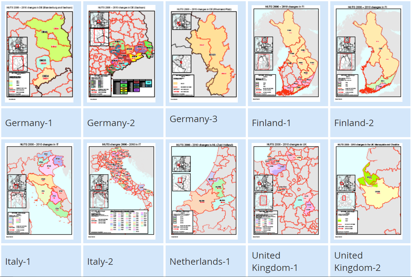
Figure 2. Changes in the NUTS system between 2006 and 2010

Despite this, Eurostat does not always recalculate in order to dock the current territorial division with historical statistics. In practice, this means that for the most current versions of NUTS, the data contain a significant number of gaps in cases where the boundaries of the regions have changed. Therefore, researchers have to independently harmonize data in order to explore sufficiently long time periods. Of course, the data recovery process is replete with assumptions, sometimes rather coarse, that allow us to evaluate statistical indicators for regions that have never existed in the past.

In addition, the work is complicated by the fact that Eurostat publishes data only for the current version of NUTS (at least I have not found where to download archived datasets - I will be grateful for the tip, if they still exist somewhere). As part of my PhD project, I conduct a regional analysis at the NUTS-2 level. To ensure the longest observation period, in 2015, when I did the main work on data harmonization, I chose the 2010 version of NUTS, on which the official regional demographic forecast EUROPOP2013 was based . In order to reproduce the results, I laid out on figshare copies of the initial data at the NUTS level about the age structures of the population and deaths downloaded in 2015.

Denmark

Some countries had to make large-scale reforms of the administrative-territorial division in order to meet the standards of NUTS. The most significant changes occurred simultaneously in Denmark in 2007 , when 271 old municipalities were transformed into 98 new ones (see the scientific article on reform ). The same reform introduced NUTS for Denmark: 98 new municipalities united in 11 NUTS-3 regions, which in turn united in 5 NUTS-2 regions. The NUTS-1 level does not stand out, which is typical for small countries like Denmark.

As far as I know, no attempts were made to restore data for NUTS regions of Denmark until 2007 at the official level. A typical map of European regions published by Eurostat for the period up to 2007 looks like this (Fig. 3) - “no data available” for the Danish regions.

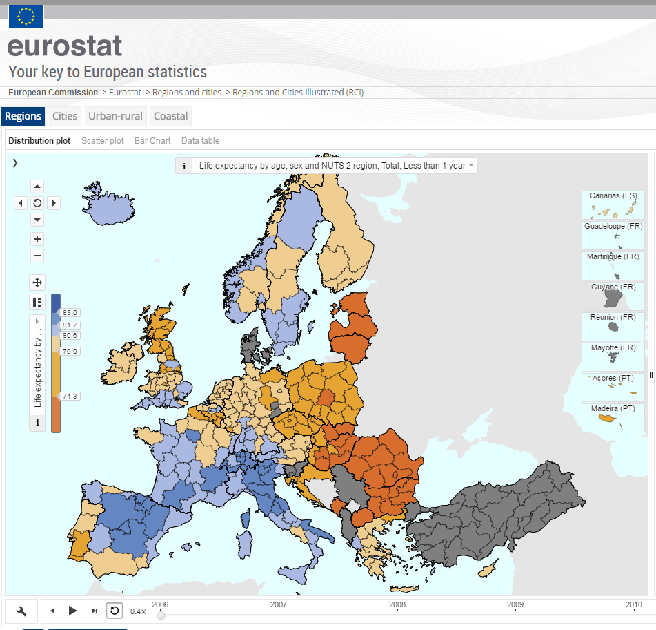
Figure 3. Life expectancy in the NUTS-2 regions of Europe, 2006; Screenshot of Eurostatov's interactive data exploratory tool

Such a lack of data is extremely surprising for a country as highly developed in many respects as Denmark. It can be quite difficult to reconcile the old and new systems of municipal division, but aggregating municipal data at much higher hierarchical levels of NUTS is not that difficult. And this is exactly what I did and I want to show in this post. I spent quite a lot of effort to find out if someone else had done this before me - much to my surprise, I did not find anything in the public domain.

The task, in essence, is to correlate the old municipalities (271) with the modern NUTS-3 regions (11) and then simply aggregate the data at the NUTS-3 level. Further, NUTS-3 is elementarily aggregated to NUTS-2. Such a task can take long evenings, especially if you take into account all the joy of messing around with the charming Danish names of the municipalities. But, fortunately, we live in the GIS era. I used GIS to almost automatically connect old municipalities with NUTS-3 regions. Further, the whole process is shown step by step with the code R.

Data

Data on the age structure of the old 271 municipalities in Denmark are taken from the official website of Statistics Denmark . The system allows you to download at once only 10K records for unregistered users and 100K after registration. Given the detail of our data, the process of uploading data is a rather tedious job. Therefore, for the tasks of my research, I downloaded the data for 2001-2006. If necessary, detailed municipal data have been available since 1979. Data downloaded by me in 2015 and slightly formatted before use are here .

The search for the spatial data file of the borders of the old Danish municipalities took considerable time. Returning to this question a year and a half later, I did not manage to find the original source of the shapefile. But I'm pretty sure I downloaded it from here . Today there is a visit notice that data is not available due to scheduled work. Copy of used shapefile here .

Finally, for the successful implementation of our plans, we need the boundaries of the NUTS-3 regions. Everything is simple - data is available on the Eurostat website ( Eurostat geodata repository ). The archived shapefile I used is called "NUTS_2010_20M_SH.zip". A sample of 11 Danish regions is here .

The geographical projection used for both shapefiles is ESPG-3044 , which is fairly standard for Denmark.

Finally, the R code preparing the session and downloading the data (I do not translate the comments on the code).

# set locale and encoding parameters to read Danish if(Sys.info()['sysname']=="Linux"){ Sys.setlocale("LC_CTYPE", "da_DK.utf8") danish_ecnoding <- "WINDOWS-1252" }else if(Sys.info()['sysname']=="Windows"){ Sys.setlocale("LC_CTYPE", "danish") danish_ecnoding <- "Danish_Denmark.1252" } # load required packages (install first if needed) library(tidyverse) # version: 1.0.0 library(ggthemes) # version: 3.3.0 library(rgdal) # version: 1.2-4 library(rgeos) # version: 0.3-21 library(RColorBrewer) # version: 1.1-2 mypal <- brewer.pal(11, "BrBG") library(fuzzyjoin) # version: 0.1.2 library(viridis) # version: 0.3.4 # load Denmark pop structures for the old municipalities df <- read_csv("https://ikashnitsky.imtqy.com/doc/misc/nuts2-denmark/BEF1A.csv.gz") # create a directory for geodata ifelse(!dir.exists("geodata"), dir.create("geodata"), "Directory already exists") # download, unzip and read Danish NUTS-3 geodata (31KB) url_nuts <- "https://ikashnitsky.imtqy.com/doc/misc/nuts2-denmark/denmark-nuts3-espg3044.tgz" path_nuts <- "geodata/denmark-nuts3-espg3044.tgz" ifelse(!file.exists(path_nuts), download.file(url_nuts, path_nuts, mode="wb"), 'file alredy exists') # If there are problems downloading the data automatically, please download it manually from # https://ikashnitsky.imtqy.com/doc/misc/nuts2-denmark/denmark-nuts3-espg3044.tgz untar(tarfile = path_nuts, exdir = "geodata") sp_nuts3 <- readOGR(dsn = "geodata/.", layer = "denmark-nuts3-espg3044") gd_nuts3 <- fortify(sp_nuts3, region = "NUTS_ID") # to the ggplot format # download, unzip and read Danish old municipal geodata (6.0MB) url_mun <- "https://ikashnitsky.imtqy.com/doc/misc/nuts2-denmark/kommune2006win1252.tgz" path_mun <- "geodata/kommune2006win1252.tgz" ifelse(!file.exists(path_mun), download.file(url_mun, path_mun, mode="wb"), 'file alredy exists') # If there are problems downloading the data automatically, please download it manually from # https://ikashnitsky.imtqy.com/doc/misc/nuts2-denmark/kommune2006utf8.tgz untar(tarfile = path_mun, exdir = "geodata") sp_mun <- readOGR(dsn = "geodata/.", layer = "kommune2006win1252", encoding = danish_ecnoding) gd_mun <- fortify(sp_mun) # coordinates of the municipalities mun_coord <- bind_cols(as.data.frame(coordinates(sp_mun)), sp_mun@data[,1:3]) %>% transmute(long = V1, lat = V2, enhedid, objectid, name = navn) 

Spatial docking

Let's first look at the map.

 ggplot()+ geom_polygon(data = gd_nuts3, aes(long, lat, group = group), color = brbg[3], fill = "grey90", size = 1)+ geom_point(data = mun_coord, aes(long, lat), color = brbg[10], size = 1)+ theme_map()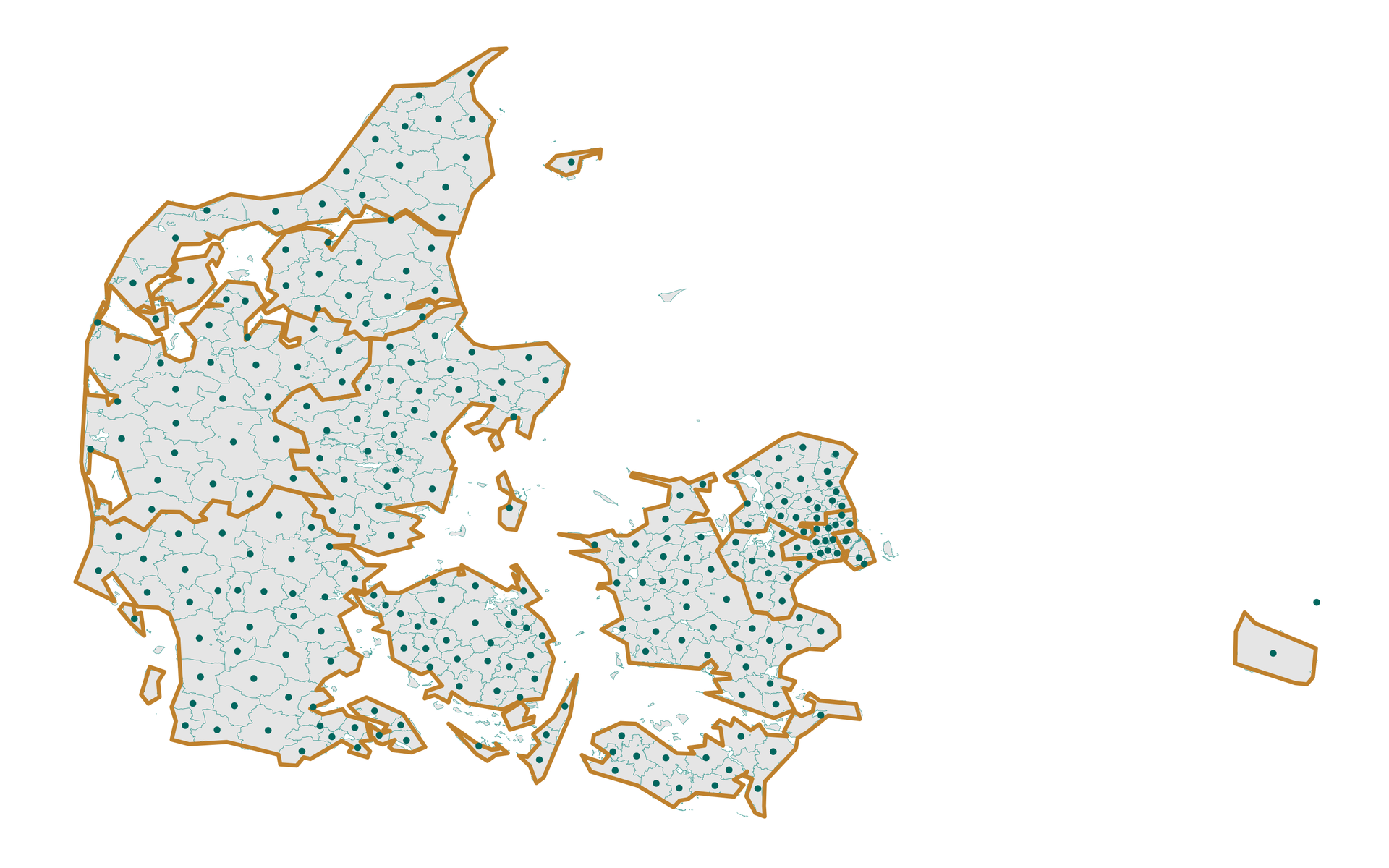 

Figure 4. Old municipalities and NUTS-3 regions of Denmark

It can be seen that the boundaries of municipalities (light blue) are much more detailed than the boundaries of the NUTS-3 regions (light brown). This is not difficult as long as the centroids of the municipalities fall within the respective NUTS-3 regions. This is true for all centroids except the easternmost point. Fast googlej tells us that this is Christiansø , a tiny island with a medieval fortress and rich history . This municipality has a special status and is not included in the NUTS system. For our further manipulations, we can safely stick it to the neighboring island of Bornholm.

To find out which centroids fall into which NUTS regions, I used the spatial overlap function ( over ) from the sp library. Here I want to thank Roger Bivand , a person without whom there would be no modern cartographic methods for R.

 # municipality coordinates to Spatial mun_centr <- SpatialPoints(coordinates(sp_mun), proj4string = CRS(proj4string(sp_nuts3))) # spatial intersection with sp::over inter <- bind_cols(mun_coord, over(mun_centr, sp_nuts3[,"NUTS_ID"])) %>% transmute(long, lat, objectid, nuts3 = as.character(NUTS_ID), nuts2 = substr(nuts3, 1, 4)) 

Check if the spatial dock is working.

 ggplot()+ geom_polygon(data = gd_mun, aes(long, lat, group = group), color = brbg[9], fill = "grey90", size = .1)+ geom_polygon(data = gd_nuts3, aes(long, lat, group = group), color = brbg[3], fill = NA, size = 1)+ geom_point(data = inter, aes(long, lat, color = nuts3), size = 1)+ geom_point(data = inter[is.na(inter$nuts3),], aes(long, lat), color = "red", size = 7, pch = 1)+ theme_map(base_size = 15)+ theme(legend.position = c(1, 1), legend.justification = c(1, 1))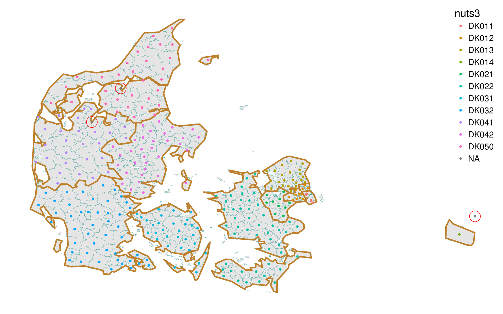 

Figure 5. Checking the spatial intersection between the old municipalities and the NUTS-3 regions of Denmark

Not bad. But there are several municipalities that fall into the “NA” category, which means that they could not find a match at the NUTS level. How many such cases do we have?

 # how many failed cases do we have sum(is.na(inter$nuts3)) 

 ## [1] 3 

 # where the intersection failed inter[is.na(inter$nuts3),] 

 ## long lat objectid nuts3 nuts2 ## 23 892474.0 6147918 46399 <NA> <NA> ## 65 504188.4 6269329 105319 <NA> <NA> ## 195 533446.8 6312770 47071 <NA> <NA> 

Only 3. I decided to fix them manually.

 # fix the three cases manually fixed <- inter fixed[fixed$objectid=="46399", 4:5] <- c("DK014", "DK01") fixed[fixed$objectid=="105319", 4:5] <- c("DK041", "DK04") fixed[fixed$objectid=="47071", 4:5] <- c("DK050", "DK05") 

Final visual check.

 ggplot()+ geom_polygon(data = gd_mun, aes(long, lat, group = group), color = brbg[9], fill = "grey90", size = .1)+ geom_polygon(data = gd_nuts3, aes(long, lat, group = group), color = brbg[3], fill = NA, size = 1)+ geom_point(data = fixed, aes(long, lat, color = nuts3), size = 1)+ theme_map(base_size = 15)+ theme(legend.position = c(1, 1), legend.justification = c(1, 1))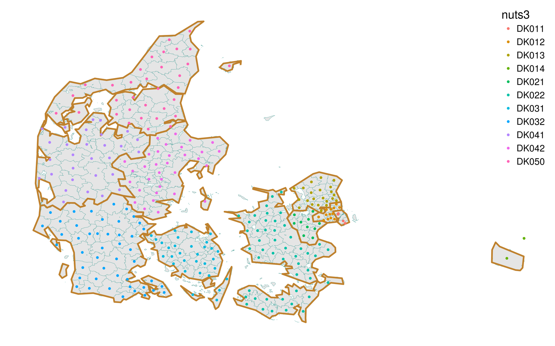 

Figure 6. Reconciliation of spatial alignment after manual adjustment for 3 municipalities

Now everything is normal.

Connect spatial and statistical data (fuzzy join)

The next task turned out to be not trivial matching of spatial and statistical data. The municipality shapefile I found did not contain the identification codes used by Statistics Denmark. Therefore, we had to connect the municipalities in the spatial and statistical datasets by name - with all the delights of Danish names and Western European coding. The names of municipalities can be written slightly differently in two datasets. And hundreds of municipalities. It would seem rather boring routine work. Not here it was! Comes to the aid of 'Fuzzy String Matching' and its excellent implementation in the fuzzyjoin library, written by the great developer David Robinson .

To begin with, I simplified the data of the names of municipalities, transferring them to the lower register, of course, in both datasets. In addition, the first attempts at docking showed that it makes sense to replace the letter “å” with an alternative spelling - “aa”. In spatial dataset, I also removed the word “Kommune” from the name of each municipality. I downloaded a tiny dataset from the Statistics Denmark website, containing the names and codes of the old municipalities.

 # simplify municipalities names mun_geo <- mun_coord %>% transmute(name = sub(x = name, " Kommune", replacement = ""), objectid) %>% mutate(name = gsub(x = tolower(name), "å", "aa")) mun_stat <- read.csv2("https://ikashnitsky.imtqy.com/doc/misc/nuts2-denmark/stat-codes-names.csv", fileEncoding = danish_ecnoding) %>% select(name) %>% separate(name, into = c("code", "name"), sep = " ", extra = "merge") %>% mutate(name = gsub("\\s*\\([^\\)]+\\)", "", x = name)) %>% mutate(name = gsub(x = tolower(name), "å", "aa")) 

We try fuzzy join.

 # first attempt fuz_joined_1 <- regex_left_join(mun_geo, mun_stat, by = "name") 

At the output we get a dataframe with 278 lines instead of 271. This means that for some municipalities from the spatial dataset more than one match was found in the statistical dataset. We find these problem cases.

 # identify more that 1 match (7 cases) and select which to drop fuz_joined_1 %>% group_by(objectid) %>% mutate(n = n()) %>% filter(n > 1) 

 ## Source: local data frame [14 x 5] ## Groups: objectid [7] ## ## name.x objectid code name.yn ## <chr> <dbl> <chr> <chr> <int> ## 1 haslev 105112 313 haslev 2 ## 2 haslev 105112 403 hasle 2 ## 3 brønderslev 47003 739 rønde 2 ## 4 brønderslev 47003 805 brønderslev 2 ## 5 hirtshals 47037 817 hals 2 ## 6 hirtshals 47037 819 hirtshals 2 ## 7 rønnede 46378 385 rønnede 2 ## 8 rønnede 46378 407 rønne 2 ## 9 hvidebæk 46268 317 hvidebæk 2 ## 10 hvidebæk 46268 681 videbæk 2 ## 11 ryslinge 46463 477 ryslinge 2 ## 12 ryslinge 46463 737 ry 2 ## 13 aarslev 46494 497 aarslev 2 ## 14 aarslev 46494 861 aars 2 

So, for 7 municipalities 2 matches were found. Not ideal matches will be thrown away at the next iteration of the fuzzy join.

Another problem is that for some municipalities there was no match at all.

 # show the non-matched cases fuz_joined_1 %>% filter(is.na(code)) 

 ## name.x objectid code name.y ## 1 faxe 105120 <NA> <NA> ## 2 nykøbing falsters 46349 <NA> <NA> ## 3 herstederne 46101 <NA> <NA> 

Since there were only three such cases, I corrected them manually in the spatial dataset so that they correspond to the names in the statistical dataset. In two cases, the discrepancy occurred due to inaccuracies in writing, and in another case, the name of the municipality changed .

 # correct the 3 non-matching geo names mun_geo_cor <- mun_geo mun_geo_cor[mun_geo_cor$name=="faxe", "name"] <- "fakse" mun_geo_cor[mun_geo_cor$name=="nykøbing falsters", "name"] <- "nykøbing f." mun_geo_cor[mun_geo_cor$name=="herstederne", "name"] <- "albertslund" 

Now we will try to dock a second time (the names in the spatial dataset have been corrected).

 # second attempt fuz_joined_2 <- regex_left_join(mun_geo_cor, mun_stat, by = "name") # drop non-perfect match fuz_joined_2 <- fuz_joined_2 %>% group_by(objectid) %>% mutate(n = n()) %>% ungroup() %>% filter(n < 2 | name.x==name.y) fuz_joined_2 <- fuz_joined_2 %>% transmute(name = name.x, objectid, code) 

Perfect. Now the last step - in the “objectid” field we attach the data on the belonging of the NUTS regions to the old statistical codes of the municipalities.

 # finally, attach the NUTS info to matched table key <- left_join(fuz_joined_2, fixed, "objectid") 

Aggregation of municipal data at NUTS levels

The previous manipulations have given us a small, but very valuable data frame, which docks the statistical code of the old municipalities with the modern NUTS regions. It remains for us to only aggregate the old data. And I attach the “key” to the statistics and aggregate from at the NUTS-3 and NUTS-2 levels.

 # finally, we only need to aggregate the old stat data df_agr <- left_join(key, df, "code") %>% filter(!is.na(name)) %>% gather("year", "value", y2001:y2006) df_nuts3 <- df_agr %>% group_by(year, sex, age, nuts3) %>% summarise(value = sum(value)) %>% ungroup() df_nuts2 <- df_agr %>% group_by(year, sex, age, nuts2) %>% summarise(value = sum(value)) %>% ungroup() 

Let’s take a sample of the working-age population (15–64) in the NUTS-3 regions of Denmark in 2001 and put this information on the map.

 # total population in 2001 by NUTS-3 regions tot_01 <- df_nuts3 %>% filter(year=="y2001") %>% group_by(nuts3) %>% summarise(tot = sum(value, na.rm = TRUE)) %>% ungroup() # working-age population in 2001 by NUTS-3 regions working_01 <- df_nuts3 %>% filter(year=="y2001", age %in% paste0("a0", 15:64)) %>% group_by(nuts3) %>% summarise(work = sum(value, na.rm = TRUE)) %>% ungroup() # calculate the shares of working age population sw_01 <- left_join(working_01, tot_01, "nuts3") %>% mutate(sw = work / tot * 100) 

 # map the shares of working age population in 2001 by NUTS-3 regions ggplot()+ geom_polygon(data = gd_nuts3 %>% left_join(sw_01, c("id" = "nuts3")), aes(long, lat, group = group, fill = sw), color = "grey50", size = 1) + scale_fill_viridis()+ theme_map(base_size = 15)+ theme(legend.position = c(1, 1), legend.justification = c(1, 1))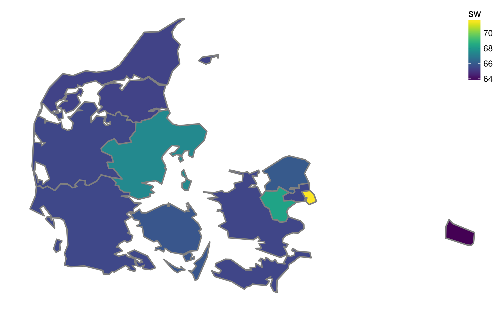 

Figure 7. The share of the working-age population (15-64) in the NUTS-3 regions of Denmark in 2001

The result looks realistic - the figure is higher in the metropolitan area and those regions where there are relatively large cities.