Deep Learning Libraries: Keras

Hi, Habr! We already talked about Theano and Tensorflow (and also a lot about what else), and today it's time to talk about Keras.

Keras originally grew up as a handy add-on to Theano. Hence, his Greek name is κέρας, which means "horn" in Greek, which, in turn, is a reference to Homer's Odyssey. Although, a lot of water has flowed since then, and Keras began to maintain Tensorflow first, and then became a part of it. However, our story will be devoted not to the difficult fate of this framework, but to its capabilities. If it is interesting to you, welcome under kat.

It is worth starting from the stove, that is, from the table of contents.

• [Installation]
• [Backends]
• [Practical example]
  
  • [Data]
  • [Model]
    
    • [Sequential API]
    • [Functional API]
  • [Preparing the model for work]
  • [Custom loss]
  • [Training and Testing]
  • [Callbacks]
    
    • [Tensorboard]
• [Advanced Graphs]
• [Conclusion]

Installation

Installing Keras is extremely easy. it is the usual python package:

pip install keras 

Now we can proceed to his analysis, but first we will talk about backends.

ATTENTION: To work with Keras, you must already have at least one of the frameworks installed - Theano or Tensorflow.

Backends

Backends are what made Keras famous and popular (among other things, which we’ll discuss below). Keras allows you to use various other frameworks as a backend. In this case, the code you write will be executed regardless of the backend used. Development began, as we have said, with Theano, but over time Tensorflow was added. Keras now works with it by default, but if you want to use Theano, then there are two options for how to do it:

1. Edit the keras.json configuration file, which lies along the path of $HOME/.keras/keras.json (or %USERPROFILE%\.keras\keras.json for Windows operating systems). We need a backend field:
   

    { "image_data_format": "channels_last", "epsilon": 1e-07, "floatx": "float32", "backend": "theano" } 

2. The second way is to set the environment variable KERAS_BACKEND , for example, like this:
   

    KERAS_BACKEND=theano python -c "from keras import backend" Using Theano backend. 

It is worth noting that work is currently underway on writing binding for CNTK from Microsoft, so after a while another available backend will appear. Watch this here .

There is also the MXNet Keras backend , which does not yet have all the functionality, but if you use MXNet, you can pay attention to this possibility.

There is also an interesting project Keras.js , which makes it possible to run the trained models of Keras from a browser on machines with a GPU.

So the Keras backends are spreading and eventually will take over the world! (But it is not exactly.)

Practical example

In previous articles, much attention was paid to the description of the work of classical models of machine learning on the frameworks described. It seems that now we can take as an example a [not very] deep neural network.

Data

Learning any model in machine learning begins with data. Keras has several training datasets inside, but they are already in a convenient form and do not allow showing the full power of Keras. Therefore we will take more crude. It will be dataset 20 newsgroups - 20 thousand news messages from Usenet groups (this is such a mail exchange system from the 1990s, akin to FIDO, which, perhaps, is a little better familiar to the reader) is approximately equally distributed in 20 categories. We will teach our network how to correctly distribute messages to these newsgroups.

 from sklearn.datasets import fetch_20newsgroups newsgroups_train = fetch_20newsgroups(subset='train') newsgroups_test = fetch_20newsgroups(subset='test') 

Here is an example of the content of the document from the training set:

Preprocessing

Keras contains tools for conveniently preprocessing texts, images and time series, in other words, the most common data types. Today we work with texts, so we need to break them into tokens and bring them into matrix form.

 tokenizer = Tokenizer(num_words=max_words) tokenizer.fit_on_texts(newsgroups_train["data"]) #         x_train = tokenizer.texts_to_matrix(newsgroups_train["data"], mode='binary') x_test = tokenizer.texts_to_matrix(newsgroups_test["data"], mode='binary') 

At the output we have got binary matrices of such sizes:

 x_train shape: (11314, 1000) x_test shape: (7532, 1000) 

The first number is the number of documents in the sample, and the second is the size of our dictionary (one thousand in this example).

We will also need to convert class labels to a matrix form for learning using cross-entropy. To do this, we will translate the class number into the so-called one-hot vector, i.e. vector consisting of zeros and one unit:

 y_train = keras.utils.to_categorical(newsgroups_train["target"], num_classes) y_test = keras.utils.to_categorical(newsgroups_test["target"], num_classes) 

At the output, we also get binary matrices of such sizes:

 y_train shape: (11314, 20) y_test shape: (7532, 20) 

As we can see, the sizes of these matrices partially coincide with the data matrices (according to the first coordinate - the number of documents in the training and test samples), and partially - not. In the second coordinate, we have the number of classes (20, as the name implies).

Everything, now we are ready to teach our network to classify news!

Model

The model in Keras can be described in two main ways:

Sequential api

The first is a consistent description of the model, for example, like this:

 model = Sequential() model.add(Dense(512, input_shape=(max_words,))) model.add(Activation('relu')) model.add(Dropout(0.5)) model.add(Dense(num_classes)) model.add(Activation('softmax')) 

or like this:

 model = Sequential([ Dense(512, input_shape=(max_words,)), Activation('relu'), Dropout(0.5), Dense(num_classes), Activation('softmax') ]) 

Functional API

Some time ago it became possible to use a functional API to create a model - the second way:

 a = Input(shape=(max_words,)) b = Dense(512)(a) b = Activation('relu')(b) b = Dropout(0.5)(b) b = Dense(num_classes)(b) b = Activation('softmax')(b) model = Model(inputs=a, outputs=b) 

There are no principal differences between the methods; choose which one you prefer.
The Model class (and the Sequential inherited from it) has a convenient interface that allows you to see which layers are included in the model — model.layers , inputs — model.inputs , and outputs — model.outputs .

Also a very convenient method for displaying and saving the model is model.to_yaml .

 backend: tensorflow class_name: Model config: input_layers: - [input_4, 0, 0] layers: - class_name: InputLayer config: batch_input_shape: !!python/tuple [null, 1000] dtype: float32 name: input_4 sparse: false inbound_nodes: [] name: input_4 - class_name: Dense config: activation: linear activity_regularizer: null bias_constraint: null bias_initializer: class_name: Zeros config: {} bias_regularizer: null kernel_constraint: null kernel_initializer: class_name: VarianceScaling config: {distribution: uniform, mode: fan_avg, scale: 1.0, seed: null} kernel_regularizer: null name: dense_10 trainable: true units: 512 use_bias: true inbound_nodes: - - - input_4 - 0 - 0 - {} name: dense_10 - class_name: Activation config: {activation: relu, name: activation_9, trainable: true} inbound_nodes: - - - dense_10 - 0 - 0 - {} name: activation_9 - class_name: Dropout config: {name: dropout_5, rate: 0.5, trainable: true} inbound_nodes: - - - activation_9 - 0 - 0 - {} name: dropout_5 - class_name: Dense config: activation: linear activity_regularizer: null bias_constraint: null bias_initializer: class_name: Zeros config: {} bias_regularizer: null kernel_constraint: null kernel_initializer: class_name: VarianceScaling config: {distribution: uniform, mode: fan_avg, scale: 1.0, seed: null} kernel_regularizer: null name: dense_11 trainable: true units: !!python/object/apply:numpy.core.multiarray.scalar - !!python/object/apply:numpy.dtype args: [i8, 0, 1] state: !!python/tuple [3, <, null, null, null, -1, -1, 0] - !!binary | FAAAAAAAAAA= use_bias: true inbound_nodes: - - - dropout_5 - 0 - 0 - {} name: dense_11 - class_name: Activation config: {activation: softmax, name: activation_10, trainable: true} inbound_nodes: - - - dense_11 - 0 - 0 - {} name: activation_10 name: model_1 output_layers: - [activation_10, 0, 0] keras_version: 2.0.2 

This allows you to save models in a human-readable form, as well as instantiate models from the following description:

 from keras.models import model_from_yaml yaml_string = model.to_yaml() model = model_from_yaml(yaml_string) 

It is important to note that the model saved in text form (by the way, it is possible to save also in JSON) does not contain weights. To save and load weights, use the save_weights and load_weights respectively.

Model visualization

You can not ignore the visualization. Keras has built-in visualization for models:

 from keras.utils import plot_model plot_model(model, to_file='model.png', show_shapes=True) 

This code will save the following image under the name model.png :

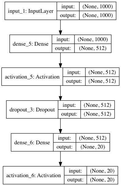
Here we additionally display the sizes of the inputs and outputs for the layers. None , the first in a tuple of sizes, is the dimension of the batch. Since costs None , the batch can be arbitrary.

If you want to display it in a jupyter laptop, you need a slightly different code:

 from IPython.display import SVG from keras.utils.vis_utils import model_to_dot SVG(model_to_dot(model, show_shapes=True).create(prog='dot', format='svg')) 

It is important to note that for visualization you need the graphviz package, as well as the python pydot package. There is a subtle point that the pydot package will not work from the repository for the visualization to work correctly, you need to get its updated version of pydot-ng .

 pip install pydot-ng 

The graphviz package in Ubuntu is set up like this (in other Linux distributions it is the same):

 apt install graphviz 

On MacOS (using the HomeBrew package system):

 brew install graphviz 

Installation instructions for Windows can be found here .

Preparing the model for work

So, we have formed our model. Now you need to prepare it for work:

 model.compile(loss='categorical_crossentropy', optimizer='adam', metrics=['accuracy']) 

What do the parameters of the compile function mean? loss is a function of error, in our case it is cross-entropy, just for it we prepared our labels in the form of matrices; optimizer is the optimizer used, there might be a regular stochastic gradient descent, but Adam shows the best convergence on this problem; Metrics - metrics by which the quality of a model is considered, in our case, is accuracy (accuracy), that is, the proportion of correctly guessed answers.

Custom loss

Although Keras contains most of the popular error functions, your task may require something unique. To make your own loss , you need a bit: just define a function that takes vectors of correct and predicted answers and gives one number to the output. For training we will do our function of calculating the cross-entropy. To make it something different, we introduce the so-called clipping - cutting the values ​​of the vector above and below. Yes, another important note: non-standard loss may be necessary to describe in terms of the underlying framework, but we can do with Keras tools.

 from keras import backend as K epsilon = 1.0e-9 def custom_objective(y_true, y_pred): '''Yet another cross-entropy''' y_pred = K.clip(y_pred, epsilon, 1.0 - epsilon) y_pred /= K.sum(y_pred, axis=-1, keepdims=True) cce = categorical_crossentropy(y_pred, y_true) return cce 

Here, y_true and y_pred are tensors from Tensorflow, so Tensorflow functions are used to process them.

To use another loss function, it is enough to change the loss parameter of the compile function, passing the object to our loss function (in the python, functions are also objects, although this is a completely different story):

 model.compile(loss=custom_objective, optimizer='adam', metrics=['accuracy']) 

Training and Testing

Finally, it's time to learn the model:

 history = model.fit(x_train, y_train, batch_size=batch_size, epochs=epochs, verbose=1, validation_split=0.1) 

The fit method does just that. It accepts a training sample together with tags - x_train and y_train , y_train size, which limits the number of examples given at a time, the number of epochs learning epochs (one epoch is a fully completed training sample once), as well as what proportion of the training sample to give for validation is validation_split .

Returns this method. history is an error history at each step of learning.

Finally, testing. The evaluate method receives a test sample at the entrance along with labels for it. The metric was set during preparation for work, so nothing else is needed. (But we will also indicate the size of the batch).

 score = model.evaluate(x_test, y_test, batch_size=batch_size) 

Callbacks

It is also necessary to say a few words about such an important feature of Keras, as kolbek. Through them implemented a lot of useful functionality. For example, if you have been training your network for a very long time, you need to understand when it’s time to stop, if the error on your dataset has ceased to decrease. In English, the described functionality is called "early stopping". Let's see how we can apply it when training our network:

 from keras.callbacks import EarlyStopping early_stopping=EarlyStopping(monitor='value_loss') history = model.fit(x_train, y_train, batch_size=batch_size, epochs=epochs, verbose=1, validation_split=0.1, callbacks=[early_stopping]) 

Do an experiment and check how quickly early stopping works in our example?

Tensorboard

Even as a callback, you can use the preservation of logs in a format convenient for Tensorboard (there was a conversation about it in the article about Tensorflow, in short it is a special utility for processing and visualizing information from Tensorflow logs).

 from keras.callbacks import TensorBoard tensorboard=TensorBoard(log_dir='./logs', write_graph=True) history = model.fit(x_train, y_train, batch_size=batch_size, epochs=epochs, verbose=1, validation_split=0.1, callbacks=[tensorboard]) 

After the training is completed (or even in the process!), You can run Tensorboard , specifying the absolute path to the directory with logs:

 tensorboard --logdir=/path/to/logs 

There you can see, for example, how the target metric changed on the validation sample:

(By the way, here you can see that our network is being retrained.)

Advanced graphs

Now consider building a slightly more complex computation graph. A neural network can have multiple inputs and outputs; input data can be transformed by various mappings. To reuse parts of complex graphs (in particular, for transfer learning ), it makes sense to describe the model in a modular style, allowing you to conveniently extract, save and apply to the new input data pieces of the model.

It is most convenient to describe the model by mixing both methods - the Functional API and the Sequential API described earlier.

Consider this approach on the example of the model Siamese Network. Similar models are widely used in practice to obtain vector representations with useful properties. For example, a similar model can be used to learn how to display photos of faces in a vector, so that vectors for similar faces will be close to each other. In particular, image search applications such as FindFace use this.

An illustration of the model can be seen in the diagram:

Here, the G function turns the input image into a vector, after which the distance between the vectors for a pair of images is calculated. If the pictures are from the same class, the distance should be minimized; if from different ones - maximized.

After such a neural network is trained, we will be able to present an arbitrary picture as a vector G(x) and use this representation either to search for the nearest images or as a vector of signs for other machine learning algorithms.

We will describe the model in the code accordingly, making it as easy as possible to extract and reuse parts of the neural network.

First, we define a function on Keras that displays the input vector.

 def create_base_network(input_dim): seq = Sequential() seq.add(Dense(128, input_shape=(input_dim,), activation='relu')) seq.add(Dropout(0.1)) seq.add(Dense(128, activation='relu')) seq.add(Dropout(0.1)) seq.add(Dense(128, activation='relu')) return seq 

Note: we described the model using the Sequential API , however we wrapped its creation into a function. Now we can create such a model by calling this function and apply it using the Functional API to the input data:

 base_network = create_base_network(input_dim) input_a = Input(shape=(input_dim,)) input_b = Input(shape=(input_dim,)) processed_a = base_network(input_a) processed_b = base_network(input_b) 

Now the processed_a and processed_b variables processed_a vector representations obtained by applying a network, defined earlier, to the input data.

It is necessary to calculate the distance between them. To do this, Keras has a Lambda wrapper function that represents any expression as a layer. Do not forget that we process the data in batch data, so that all tensors always have an extra dimension, which is responsible for the size of the batch.

 from keras import backend as K def euclidean_distance(vects): x, y = vects return K.sqrt(K.sum(K.square(x - y), axis=1, keepdims=True)) distance = Lambda(euclidean_distance)([processed_a, processed_b]) 

Great, we got the distance between the internal views, now it remains to collect the entrances and the distance in one model.

 model = Model([input_a, input_b], distance) 

Thanks to the modular structure, we can use base_network separately, which is especially useful after training the model. How can I do that? Let's look at the layers of our model:

 >>> model.layers [<keras.engine.topology.InputLayer object at 0x7f238fdacb38>, <keras.engine.topology.InputLayer object at 0x7f238fdc34a8>, <keras.models.Sequential object at 0x7f239127c3c8>, <keras.layers.core.Lambda object at 0x7f238fddc4a8>] 

We see the third object in the list of the type models.Sequential . models.Sequential . This is the model that displays the input image in the vector. To extract and use it as a full-fledged model (you can train, validate, embed in another graph) you just need to pull it out of the list of layers:

 >>> embedding_model = model.layers[2] >>> embedding_model.layers [<keras.layers.core.Dense object at 0x7f23c4e557f0>, <keras.layers.core.Dropout object at 0x7f238fe97908>, <keras.layers.core.Dense object at 0x7f238fe44898>, <keras.layers.core.Dropout object at 0x7f238fe449e8>, <keras.layers.core.Dense object at 0x7f238fe01f60>] 

For example, for a Siamese network already trained on MNIST data with a base_model output of two, you can visualize vector representations as follows:

Load the data and bring the images of size 28x28 to flat vectors.

 (x_train, y_train), (x_test, y_test) = mnist.load_data() x_test = x_test.reshape(10000, 784) 

Display the images using the previously extracted model:

 embeddings = embedding_model.predict(x_test) 

Now in the embeddings are two-dimensional vectors, they can be drawn on the plane: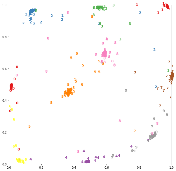

A full example of the Siamese network can be seen here .

Conclusion

That's it, we made the first models on Keras! We hope that the opportunities provided to them interested you, so that you will use it in your work.

It's time to discuss the pros and cons of Keras. The obvious advantages include the simplicity of creating models, which translates into high speed prototyping. For example, the authors of a recent article about satellites used exactly Keras. In general, this framework is becoming more and more popular:

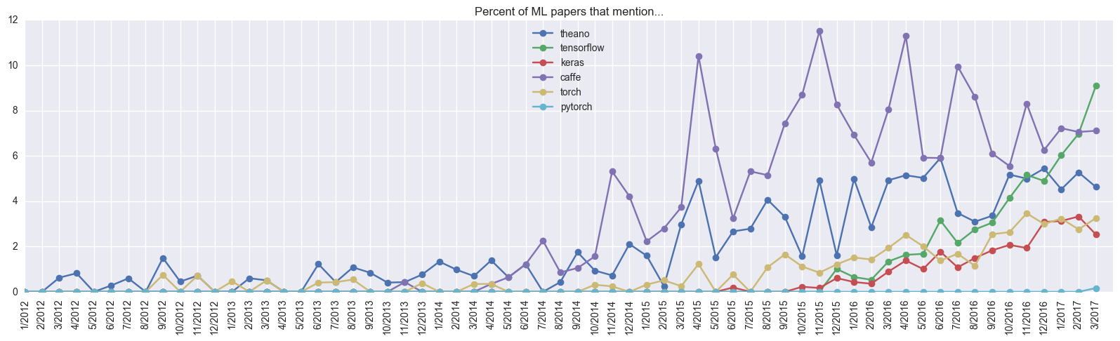
Keras caught up with Torch for a year, which has been under development for 5 years, judging by references in scientific articles. It seems his goal - ease of use - Francois Chollet (François Chollet, author Keras) achieved. Moreover, his initiative did not go unnoticed: after just a few months of development, Google invited him to do this in the team developing Tensorflow. And also with the version Tensorflow 1.2 Keras will be included in the TF (tf.keras).

Also need to say a few words about the shortcomings. Unfortunately, Keras’s idea of ​​code universality is not always fulfilled: Keras 2.0 broke compatibility with the first version, some functions were renamed differently, some moved, in general, the story is similar to the second and third python. The difference is that in the case of Keras, only the second version was chosen for development. Also, the Keras code works on Tensorflow while slower than on Theano (although for the native code, the frameworks are at least comparable ).

In general, you can recommend Keras for use when you need to quickly build and test a network for a specific task. But if you need some complicated things, like a non-standard layer or code parallelization on several GPUs, then it is better (and sometimes simply inevitable) to use the underlying framework.

Almost all the code from the article is in the form of a single laptop here . We also highly recommend you the Keras: keras.io documentation , as well as the official examples on which this article is largely based.

Post written in collaboration with Wordbearer .