Open machine learning course. Theme 6. Construction and selection of signs

The Open Data Science community welcomes course participants!

As part of the course, we already met several key machine learning algorithms. However, before moving on to more sophisticated algorithms and approaches, I would like to take a step aside and talk about preparing data for training the model. The well-known principle of garbage in - garbage out is 100% applicable to any machine learning task; Any experienced analyst can recall examples from practice when a simple model trained on well-prepared data performed better than a smart ensemble built on insufficiently pure data.

UPD: now the course is in English under the brand mlcourse.ai with articles on Medium, and materials on Kaggle ( Dataset ) and on GitHub .

List of articles series

In today's article, I would like to briefly describe three similar, but different tasks:

feature extraction and feature engineering - turning data that is specific to the subject area into vectors that are understandable for the model;
feature transformation - data transformation to improve the accuracy of the algorithm;
feature selection - cutting off unnecessary features.

Separately, I note that in this article there will be almost no formulas, but there will be relatively a lot of code.

In some examples, datasets will be used from the company Renthop , used in the Two Sigma Connect: Rental Listing Inquires competition on Kaggle. In this problem, you need to predict the popularity of ads for real estate rental, i.e. solve the problem of classification into three classes ['low', 'medium', 'high'] . To evaluate the solution, the log loss metric is used (the smaller the better). Those who do not have an account on Kaggle, will have to register; also for downloading data you need to accept the rules of competition.

 #        train.json.zip  Kaggle    import json import pandas as pd #     Renthop with open('train.json', 'r') as raw_data: data = json.load(raw_data) df = pd.DataFrame(data)

Feature Extraction

In life, data rarely comes in the form of ready-made matrices, so any task begins with the extraction of signs. Sometimes, of course, it is enough to read the csv file and convert it to numpy.array , but these are happy exceptions. Let's look at some of the popular data types from which to extract attributes.

Texts

The text is the most obvious example of data in a free format; There are enough methods of working with text so that they do not fit into one article. Nevertheless, we’ll go over the most popular ones.

Before working with the text, it must be tokenized. Tokenization involves splitting the text into tokens - in the simplest case, these are just words. But, by making it too simple a regular schedule ("in the forehead"), we can lose some of the meaning: "Nizhny Novgorod" is not two tokens, but one. But the call "steal, kill!" can be divided into two tokens in vain. There are ready tokenizers that take into account the peculiarities of the language, but they can be wrong, especially if you work with specific texts (professional vocabulary, jargon, typos).

After tokenization in most cases, you need to think about reduction to normal form. We are talking about stemming and / or lemmatization - these are similar processes used to process word forms. You can read about the difference between them here .

So, we turned the document into a sequence of words, you can begin to turn them into vectors. The simplest approach is called Bag of Words: we create a vector with a length in the dictionary, for each word we count the number of entries in the text and substitute this number for the corresponding position in the vector. In code, it looks even simpler than in words:

Bag of Words without extra libraries

 from functools import reduce import numpy as np texts = [['i', 'have', 'a', 'cat'], ['he', 'have', 'a', 'dog'], ['he', 'and', 'i', 'have', 'a', 'cat', 'and', 'a', 'dog']] dictionary = list(enumerate(set(reduce(lambda x, y: x + y, texts)))) def vectorize(text): vector = np.zeros(len(dictionary)) for i, word in dictionary: num = 0 for w in text: if w == word: num += 1 if num: vector[i] = num return vector for t in texts: print(vectorize(t))

Also, the idea is well illustrated with a picture:

This is an extremely naive implementation. In real life, you need to take care of the stop words, the maximum dictionary size, the effective data structure (usually text data is converted into sparse vectors) ...

Using algorithms like Vag of Words, we lose the order of words in the text, which means that the texts "i have no cows" and "no, i have cows" will be identical after vectorization, although they are opposite semantically. To avoid this problem, you can take a step back and change the approach to tokenization: for example, use N-grams (combinations of N consecutive terms).

Check in practice

 In : from sklearn.feature_extraction.text import CountVectorizer In : vect = CountVectorizer(ngram_range=(1,1)) In : vect.fit_transform(['no i have cows', 'i have no cows']).toarray() Out: array([[1, 1, 1], [1, 1, 1]], dtype=int64) In : vect.vocabulary_ Out: {'cows': 0, 'have': 1, 'no': 2} In : vect = CountVectorizer(ngram_range=(1,2)) In : vect.fit_transform(['no i have cows', 'i have no cows']).toarray() Out: array([[1, 1, 1, 0, 1, 0, 1], [1, 1, 0, 1, 1, 1, 0]], dtype=int64) In : vect.vocabulary_ Out: {'cows': 0, 'have': 1, 'have cows': 2, 'have no': 3, 'no': 4, 'no cows': 5, 'no have': 6}

Also note that it is not necessary to operate with words: in some cases it is possible to generate N-grams from letters (for example, such an algorithm will take into account the similarity of related words or typos).

 In : from scipy.spatial.distance import euclidean In : vect = CountVectorizer(ngram_range=(3,3), analyzer='char_wb') In : n1, n2, n3, n4 = vect.fit_transform(['', '', '', '']).toarray() In : euclidean(n1, n2) Out: 3.1622776601683795 In : euclidean(n2, n3) Out: 2.8284271247461903 In : euclidean(n3, n4) Out: 3.4641016151377544

The development of the Bag of Words idea: words that are rarely found in the corpus (in all the documents considered in this dataset), but are present in this particular document, may turn out to be more important. Then it makes sense to increase the weight of more specific words, in order to separate them from general topics. This approach is called TF-IDF, you can’t write it in ten lines anymore, so those who are interested can get acquainted with the details in external sources like wiki . The default option is:

i d f (t, D) = l o g f r a c m i d D m i d d f (d, t) + 1

$idf (t, D) = \ log \ frac {\ mid D \ mid} {df (d, t) + 1}$

t f i d f (t, d, D) = t f (t, d) t i m e s i d f (t, D)

$tfidf (t, d, D) = tf (t, d) \ times idf (t, D)$

Analogs of Bag of words can also be found outside of word problems: for example, bag of sites in a competition that we hold is Catch Me If You Can. You can search for other examples - bag of apps , bag of events .

Using such algorithms, you can get quite a working solution to a simple problem, such a baseline. However, for non-lovers of the classics, there are newer approaches. The most popular method of the new wave is Word2Vec, but there are also alternatives (Glove, Fasttext ...).

Word2Vec is a special case of Word Embedding algorithms. Using Word2Vec and similar models, we can not only vectorize words into a space of large dimension (usually several hundred), but also compare their semantic proximity. A classic example of operations on vectorized views: king - man + woman = queen.

It should be understood that this model, of course, does not have an understanding of words, but simply tries to place vectors in such a way that words used in the general context are located close to each other. If this is not taken into account, then you can come up with many curiosities: for example, find the opposite of Hitler by multiplying the corresponding vector by -1.

Such models should be trained on very large data sets so that the coordinates of the vectors truly reflect the semantics of the words. To solve your problems, you can download a pre-trained model, for example, here .

Similar methods, by the way, are used in other areas (for example, in bioinformatics). From completely unexpected applications - food2vec .

Images

In working with images, everything is both simpler and more complex at the same time. Easier, because you can often not think at all and use one of the popular pre-trained networks; more difficult, because if you still need to understand in detail, then this rabbit hole will be damn deep. However, first things first.

At a time when the GPU was weaker, and the "renaissance of neural networks" had not yet happened, the generation of features from the images was a separate complex area. To work with pictures, it was necessary to work at a low level, defining, for example, angles, area boundaries, and so on. Experienced computer vision specialists could draw many parallels between older approaches and the neural network hipsterism: in particular, convolutional layers in modern networks are very similar to Haar cascades . Not being experienced in this matter, I will not even try to transfer knowledge from public sources, leave a couple of links to the skimage and SimpleCV libraries and go straight to our days.

Often, some convolution network is used for problems related to images. You can not think of the architecture and not train the network from scratch, but take the pre-trained state of the art network, the weights of which can be downloaded from open sources. To adapt it to their task, the date Cynthists practice the so-called. fine tuning: the last fully connected layers of the network “come off”, new ones are added instead, selected for a specific task, and the network is trained on new data. But if you want to simply vectorize the image for some of your purposes (for example, use some kind of non-network classifier) - just tear off the last layers and use the output of the previous layers:

 from keras.applications.resnet50 import ResNet50 from keras.preprocessing import image from scipy.misc import face import numpy as np resnet_settings = {'include_top': False, 'weights': 'imagenet'} resnet = ResNet50(**resnet_settings) img = image.array_to_img(face()) #   ! img = img.resize((224, 224)) #          x = image.img_to_array(img) x = np.expand_dims(x, axis=0) #   , ..        features = resnet.predict(x)

Classifier trained in one dataset and adapted for another by “tearing off” the last layer and adding a new one in return

However, you should not get hung up on neural network methods. Some signs generated by hands may be useful even today: for example, predicting the popularity of renting an apartment, you can assume that bright apartments attract more attention, and make a sign "average pixel value". You can get inspired by examples in the documentation of the relevant libraries .

If a text is expected in a picture, it can also be read without unfolding a complex neural network with its own hands: for example, using pytesseract .

 In : import pytesseract In : from PIL import Image In : import requests In : from io import BytesIO In : img = 'http://ohscurrent.org/wp-content/uploads/2015/09/domus-01-google.jpg' #      In : img = requests.get(img) ...: img = Image.open(BytesIO(img.content)) ...: text = pytesseract.image_to_string(img) ...: In : text Out: 'Google'

We must understand that pytesseract is far from a panacea:

 #       Renthop In : img = requests.get('https://photos.renthop.com/2/8393298_6acaf11f030217d05f3a5604b9a2f70f.jpg') ...: img = Image.open(BytesIO(img.content)) ...: pytesseract.image_to_string(img) ...: Out: 'Cunveztible to 4}»'

Another case where neural networks will not help is to extract traits from the meta-information. But EXIF can store a lot of useful information: the manufacturer and model of the camera, the resolution, the use of flash, the geo-coordinates of the survey, the software used for processing and much more.

Geodata

Geographic data is not so often encountered in tasks, but it is also useful to master the basic techniques for working with them, especially since there are also enough ready-made solutions in this area.

Geodata are most often presented in the form of addresses or pairs "latitude + longitude", i.e. points. Depending on the task, you may need two operations opposite to each other: geocoding (recovery of a point from an address) and reverse geocoding (vice versa). Both are possible with external APIs like Google Maps or OpenStreetMap. Different geocoders have their own characteristics, the quality varies from region to region. Fortunately, there are universal libraries like geopy , which act as wrappers for many external services.

If there is a lot of data, it is easy to rest against the limits of external APIs. Yes, and receiving information via HTTP is not always the best solution for speed. Therefore, it is worth bearing in mind the possibility of using the local version of OpenStreetMap.

If there is little data, there is enough time, and there is no desire to extract the tricked signs, then you can not bother with OpenStreetMap and use reverse_geocoder :

 In : import reverse_geocoder as revgc In : revgc.search((df.latitude, df.longitude)) Loading formatted geocoded file... Out: [OrderedDict([('lat', '40.74482'), ('lon', '-73.94875'), ('name', 'Long Island City'), ('admin1', 'New York'), ('admin2', 'Queens County'), ('cc', 'US')])]

Working with geocoding, we must not forget that the addresses may contain typos, respectively, it is worth spending time cleaning. There is usually less typo in the coordinates, but not everything is good with them: GPS can “make noise” by the nature of data, and in some places (tunnels, blocks of skyscrapers ...) is pretty strong. If the data source is a mobile device, it is worth considering that in some cases geolocation is not determined by GPS, but by WiFi networks in the area, which leads to holes in space and teleportation: one of Chicago may suddenly turn out to be a set of points describing a journey through Manhattan. .

Teleportation hypotheses

WiFi location tracking is based on a combination of SSID and MAC addresses, which can coincide at completely different points (for example, the federal provider has standardized the firmware of routers to within the MAC address and places them in different cities). There are more trivial reasons, like moving a company with their routers to another office.

The point is usually not in the open field, but among the infrastructure - here you can give free rein to your imagination and begin to invent signs using life experience and knowledge of the domain area. The proximity of the point to the metro, the number of floors of the building, the distance to the nearest store, the number of ATMs in a radius - within the framework of one task, you can come up with dozens of signs and extract them from various external sources. For tasks outside the urban infrastructure, signs from more specific sources may be useful: for example, elevation above sea level.

If two or more points are interconnected, it may be worthwhile to extract the signs from the route between them. It will be useful and the distance (it is worth looking at the great circle distance, and the "fair" distance, calculated on the road graph), and the number of turns along with the ratio of left and right, and the number of traffic lights, junctions, bridges. For example, in one of my tasks, a sign that I called “road complexity” showed itself quite well - the distance calculated by the graph and divided by GCD.

date and time

It would seem that work with the date and time should be standardized due to the prevalence of relevant signs, but the pitfalls remain.

Let's start with the days of the week - they are easy to turn into 7 dummy variables using one-hot coding. In addition, it is useful to select a separate sign for the weekend.

 df['dow'] = df['created'].apply(lambda x: x.date().weekday()) df['is_weekend'] = df['created'].apply(lambda x: 1 if x.date().weekday() in (5, 6) else 0)

In some tasks, additional calendar features may be needed: for example, cash withdrawal may be tied to the day of salary issuance, and the purchase of a travel card - by the beginning of the month. And in a good way, working with time data, you need to have on hand a calendar with public holidays, abnormal weather conditions and other important events.

Professional unfamiliar humor

What do Chinese New Year, New York Marathon, Gay Pride Parade and Trump's inauguration have in common?
They all need to make a calendar of potential anomalies.

But with an hour (minute, day of the month ...) everything is not so rosy. If we use the hour as a real variable, we slightly contradict the nature of the data: 0 <23, although 02.01 0:00:00> 01.01 23:00:00. For some tasks, this may be critical. If you encode them as categorical variables, you can produce a bunch of signs and lose information about proximity: the difference between 22 and 23 will be the same as between 22 and 7.

There are more esoteric approaches to such data. For example, a projection on a circle with the subsequent use of two coordinates.

 def make_harmonic_features(value, period=24): value *= 2 * np.pi / period return np.cos(value), np.sin(value)

This transformation preserves the distance between points, which is important for some algorithms based on distance (kNN, SVM, k-means ...)

 In : from scipy.spatial import distance In : euclidean(make_harmonic_features(23), make_harmonic_features(1)) Out: 0.5176380902050424 In : euclidean(make_harmonic_features(9), make_harmonic_features(11)) Out: 0.5176380902050414 In : euclidean(make_harmonic_features(9), make_harmonic_features(21)) Out: 2.0

However, the difference between such coding methods can usually be caught only in the third decimal place in the metric, not earlier.

Time series, web and more

I did not have enough time to work with the time series, so I will leave a link to the library to automatically generate the signs from the time series and go on.

If you work with the web, then you usually have information about the user's User Agent. This is a storehouse of information.
First, from there, first of all, you need to extract the operating system. Second, make the sign is_mobile . Third, look at the browser.

Example of extracting traits from user agent

 In : ua = 'Mozilla/5.0 (X11; Linux x86_64) AppleWebKit/537.36 (KHTML, like Gecko) Ubuntu Chromium/56.0.2924.76 Chrome/ ...: 56.0.2924.76 Safari/537.36' In : import user_agents In : ua = user_agents.parse(ua) In : ua.is_bot Out: False In : ua.is_mobile Out: False In : ua.is_pc Out: True In : ua.os.family Out: 'Ubuntu' In : ua.os.version Out: () In : ua.browser.family Out: 'Chromium' In : ua.os.version Out: () In : ua.browser.version Out: (56, 0, 2924)

As in other domain domains, you can think up your own attributes based on conjectures about the nature of the data. At the time of this writing, Chromium 56 was new, and after a while this version of the browser can only be saved by those who haven’t rebooted this browser for a long time. Why, then, do not enter the sign "lagging behind the latest version of the browser"?

In addition to the OS and browser, you can look at the referrer (not always available), http_accept_language, and other meta-information.

The next most useful information is an IP address from which you can extract at least a country, and preferably another city, provider, connection type (mobile / landline). You need to understand that there are a variety of proxies and outdated databases, so a sign may contain noise. Network administration gurus may try to extract even more advanced features: for example, make assumptions about the use of VPN . By the way, it’s nice to combine data from the IP address with http_accept_language: if the user sits at the Chilean proxy, and the browser locale is ru_RU, something here is unclean and worthy of one in the corresponding column in the table ( is_traveler_or_proxy_user ).

In general, there are so many domain specificities in a particular area that it does not fit in one head. Therefore, I urge dear readers to share their experiences and tell in comments about the extraction and generation of signs in their work.

Feature transformations

Normalization and distribution change

Monotone conversion of features is critical for some algorithms and does not affect others. , ( , ) – / , .

: np.log , np.float64 . , ; - . , . ( ).

, : , : (-1, 1), – .

: , – . 5, .

– Standart Scaling ( Z-score normalization).

z = \frac{x - μ}{σ}

$\large z = \frac{x – \mu}{\sigma}$

StandartScaling ...

 In : from sklearn.preprocessing import StandardScaler In : from scipy.stats import beta In : from scipy.stats import shapiro In : data = beta(1, 10).rvs(1000).reshape(-1, 1) In : shapiro(data) Out: (0.8783774375915527, 3.0409122263582326e-27) #  , p-value In : shapiro(StandardScaler().fit_transform(data)) Out: (0.8783774375915527, 3.0409122263582326e-27) #   p-value

… -

 In : data = np.array([1, 1, 0, -1, 2, 1, 2, 3, -2, 4, 100]).reshape(-1, 1).astype(np.float64) In : StandardScaler().fit_transform(data) Out: array([[-0.31922662], [-0.31922662], [-0.35434155], [-0.38945648], [-0.28411169], [-0.31922662], [-0.28411169], [-0.24899676], [-0.42457141], [-0.21388184], [ 3.15715128]]) In : (data – data.mean()) / data.std() Out: array([[-0.31922662], [-0.31922662], [-0.35434155], [-0.38945648], [-0.28411169], [-0.31922662], [-0.28411169], [-0.24899676], [-0.42457141], [-0.21388184], [ 3.15715128]])

– MinMax Scaling, ( (0, 1)).

X_{n o r m} = \frac{X - X_{m i n}}{X_{m a x} - X_{m i n}}

$\large X_{norm} = \frac{X – X_{min}}{X_{max}-X_{min}}$

 In : from sklearn.preprocessing import MinMaxScaler In : MinMaxScaler().fit_transform(data) Out: array([[ 0.02941176], [ 0.02941176], [ 0.01960784], [ 0.00980392], [ 0.03921569], [ 0.02941176], [ 0.03921569], [ 0.04901961], [ 0. ], [ 0.05882353], [ 1. ]]) In : (data – data.min()) / (data.max() – data.min()) Out: array([[ 0.02941176], [ 0.02941176], [ 0.01960784], [ 0.00980392], [ 0.03921569], [ 0.02941176], [ 0.03921569], [ 0.04901961], [ 0. ], [ 0.05882353], [ 1. ]])

StandartScaling MinMax Scaling - . , , – StandartScaling. MinMax Scaling , (0, 255).

, , , :

 In : from scipy.stats import lognorm In : data = lognorm(s=1).rvs(1000) In : shapiro(data) Out: (0.05714237689971924, 0.0) In : shapiro(np.log(data)) Out: (0.9980740547180176, 0.3150389492511749)

, , , .. , – . , , , . - ( – -) - , ; , – np.log(x + const) .

-. , – QQ . , .

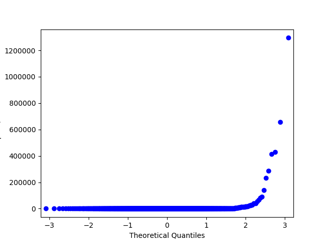
 In : import statsmodels.api as sm #   price   Renthop         In : price = df.price[(df.price <= 20000) & (df.price > 500)] In : price_log = np.log(price) In : price_mm = MinMaxScaler().fit_transform(price.values.reshape(-1, 1).astype(np.float64)).flatten() #  ,  sklearn   warning- In : price_z = StandardScaler().fit_transform(price.values.reshape(-1, 1).astype(np.float64)).flatten() In : sm.qqplot(price_log, loc=price_log.mean(), scale=price_log.std()).savefig('qq_price_log.png') In : sm.qqplot(price_mm, loc=price_mm.mean(), scale=price_mm.std()).savefig('qq_price_mm.png') In : sm.qqplot(price_z, loc=price_z.mean(), scale=price_z.std()).savefig('qq_price_z.png')

QQ StandartScaler.

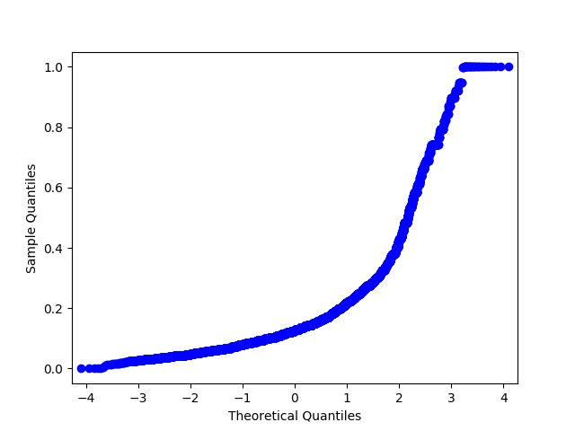
QQ MinMaxScaler.

QQ . !

, - . , Renthop, ( - ), .

 In : from demo import get_data In : x_data, y_data = get_data() In : x_data.head(5) Out: bathrooms bedrooms price dishwasher doorman pets \ 10 1.5 3 8.006368 0 0 0 10000 1.0 2 8.606119 0 1 1 100004 1.0 1 7.955074 1 0 1 100007 1.0 1 8.094073 0 0 0 100013 1.0 4 8.116716 0 0 0 air_conditioning parking balcony bike ... stainless \ 10 0 0 0 0 ... 0 10000 0 0 0 0 ... 0 100004 0 0 0 0 ... 0 100007 0 0 0 0 ... 0 100013 0 0 0 0 ... 0 simplex public num_photos num_features listing_age room_dif \ 10 0 0 5 0 278 1.5 10000 0 0 11 57 290 1.0 100004 0 0 8 72 346 0.0 100007 0 0 3 22 345 0.0 100013 0 0 3 7 335 3.0 room_sum price_per_room bedrooms_share 10 4.5 666.666667 0.666667 10000 3.0 1821.666667 0.666667 100004 2.0 1425.000000 0.500000 100007 2.0 1637.500000 0.500000 100013 5.0 670.000000 0.800000 [5 rows x 46 columns] In : x_data = x_data.values In : from sklearn.linear_model import LogisticRegression In : from sklearn.ensemble import RandomForestClassifier In : from sklearn.model_selection import cross_val_score In : from sklearn.feature_selection import SelectFromModel In : cross_val_score(LogisticRegression(), x_data, y_data, scoring='neg_log_loss').mean() /home/arseny/.pyenv/versions/3.6.0/lib/python3.6/site-packages/sklearn/linear_model/base.py:352: RuntimeWarning: overflow encountered in exp np.exp(prob, prob) # , -   ! -  ,    Out: -0.68715971821885724 In : from sklearn.preprocessing import StandardScaler In : cross_val_score(LogisticRegression(), StandardScaler().fit_transform(x_data), y_data, scoring='neg_log_loss').mean() /home/arseny/.pyenv/versions/3.6.0/lib/python3.6/site-packages/sklearn/linear_model/base.py:352: RuntimeWarning: overflow encountered in exp np.exp(prob, prob) Out: -0.66985167834479187 # !  ! In : from sklearn.preprocessing import MinMaxScaler In : cross_val_score(LogisticRegression(), MinMaxScaler().fit_transform(x_data), y_data, scoring='neg_log_loss').mean() ...: Out: -0.68522489913898188 # a    –  :(

(Interactions)

, ; , .

Two Sigma Connect: Rental Listing Inquires. . , , – , .

 rooms = df["bedrooms"].apply(lambda x: max(x, .5)) #    ; .5      df["price_per_bedroom"] = df["price"] / rooms

. , , , . , - : , ( )[ https://habrahabr.ru/company/ods/blog/322076/ ] (. sklearn.preprocessing.PolynomialFeatures ) .

" ", . , , . python : pandas.DataFrame.fillna sklearn.preprocessing.Imputer .

. :

"n/a" ( );
( , );
, - ( , , .. );
(, ) – .

- df = df.fillna(0) . : , ; .

(Feature selection)

? - , . : , . , – , . – ( ) , .

– , , .. . , , , . , .

 In : from sklearn.feature_selection import VarianceThreshold In : from sklearn.datasets import make_classification In : x_data_generated, y_data_generated = make_classification() In : x_data_generated.shape Out: (100, 20) In : VarianceThreshold(.7).fit_transform(x_data_generated).shape Out: (100, 19) In : VarianceThreshold(.8).fit_transform(x_data_generated).shape Out: (100, 18) In : VarianceThreshold(.9).fit_transform(x_data_generated).shape Out: (100, 15)

, .

 In : from sklearn.feature_selection import SelectKBest, f_classif In : x_data_kbest = SelectKBest(f_classif, k=5).fit_transform(x_data_generated, y_data_generated) In : x_data_varth = VarianceThreshold(.9).fit_transform(x_data_generated) In : from sklearn.linear_model import LogisticRegression In : from sklearn.model_selection import cross_val_score In : cross_val_score(LogisticRegression(), x_data_generated, y_data_generated, scoring='neg_log_loss').mean() Out: -0.45367136377981693 In : cross_val_score(LogisticRegression(), x_data_kbest, y_data_generated, scoring='neg_log_loss').mean() Out: -0.35775228616521798 In : cross_val_score(LogisticRegression(), x_data_varth, y_data_generated, scoring='neg_log_loss').mean() Out: -0.44033042718359772

, . , , , .

: - baseline , . : - "" (, Random Forest) Lasso , . : , .

 from sklearn.datasets import make_classification from sklearn.linear_model import LogisticRegression from sklearn.ensemble import RandomForestClassifier from sklearn.feature_selection import SelectFromModel from sklearn.model_selection import cross_val_score from sklearn.pipeline import make_pipeline x_data_generated, y_data_generated = make_classification() pipe = make_pipeline(SelectFromModel(estimator=RandomForestClassifier()), LogisticRegression()) lr = LogisticRegression() rf = RandomForestClassifier() print(cross_val_score(lr, x_data_generated, y_data_generated, scoring='neg_log_loss').mean()) print(cross_val_score(rf, x_data_generated, y_data_generated, scoring='neg_log_loss').mean()) print(cross_val_score(pipe, x_data_generated, y_data_generated, scoring='neg_log_loss').mean()) -0.184853179322 -0.235652626736 -0.158372952933

, — .

Renthop.

 x_data, y_data = get_data() x_data = x_data.values pipe1 = make_pipeline(StandardScaler(), SelectFromModel(estimator=RandomForestClassifier()), LogisticRegression()) pipe2 = make_pipeline(StandardScaler(), LogisticRegression()) rf = RandomForestClassifier() print('LR + selection: ', cross_val_score(pipe1, x_data, y_data, scoring='neg_log_loss').mean()) print('LR: ', cross_val_score(pipe2, x_data, y_data, scoring='neg_log_loss').mean()) print('RF: ', cross_val_score(rf, x_data, y_data, scoring='neg_log_loss').mean()) LR + selection: -0.714208124619 LR: -0.669572736183 #   ! RF: -2.13486716798

, , : "", , , . Exhaustive Feature Selection .

– , . N, N , , N+1 , , . , . Sequential Feature Selection .

: , .

 In : selector = SequentialFeatureSelector(LogisticRegression(), scoring='neg_log_loss', verbose=2, k_features=3, forward=False, n_jobs=-1) In : selector.fit(x_data_scaled, y_data) In : selector.fit(x_data_scaled, y_data) [2017-03-30 01:42:24] Features: 45/3 -- score: -0.682830838803 [2017-03-30 01:44:40] Features: 44/3 -- score: -0.682779463265 [2017-03-30 01:46:47] Features: 43/3 -- score: -0.682727480522 [2017-03-30 01:48:54] Features: 42/3 -- score: -0.682680521828 [2017-03-30 01:50:52] Features: 41/3 -- score: -0.68264297879 [2017-03-30 01:52:46] Features: 40/3 -- score: -0.682607753617 [2017-03-30 01:54:37] Features: 39/3 -- score: -0.682570678346 [2017-03-30 01:56:21] Features: 38/3 -- score: -0.682536314625 [2017-03-30 01:58:02] Features: 37/3 -- score: -0.682520258804 [2017-03-30 01:59:39] Features: 36/3 -- score: -0.68250862986 [2017-03-30 02:01:17] Features: 35/3 -- score: -0.682498213174 # ".      ..." ... [2017-03-30 02:21:09] Features: 10/3 -- score: -0.68657335969 [2017-03-30 02:21:18] Features: 9/3 -- score: -0.688405548594 [2017-03-30 02:21:26] Features: 8/3 -- score: -0.690213724719 [2017-03-30 02:21:32] Features: 7/3 -- score: -0.692383588303 [2017-03-30 02:21:36] Features: 6/3 -- score: -0.695321584506 [2017-03-30 02:21:40] Features: 5/3 -- score: -0.698519960477 [2017-03-30 02:21:42] Features: 4/3 -- score: -0.704095390444 [2017-03-30 02:21:44] Features: 3/3 -- score: -0.713788301404 #

№6

, .

c UCI . Jupyter notebook - , .

Source: https://habr.com/ru/post/325422/

All Articles