Bayesian multi-armed gangsters against A / B tests

Hello colleagues. Consider the usual online experiment in some company "Mustache and Claws." She has a website that has a red button in the shape of a rectangle with rounded edges. If the user presses this button, then somewhere in the world one kitten purrs with joy. The task of the company is to maximize the purring. There is also a marketing department that diligently examines the shapes of the buttons and how they affect the conversion of hits into click-purrs. Having spent almost the entire budget of the company on unique research, the marketing department was divided into four opposing groups. Each group has its own brilliant idea of how the button should look. In general, no one is against the form of the button, but the red color annoys all marketers, and in the end four alternatives were proposed. In fact, it is not even so important what options it is, we are interested in the option that maximizes purring. Marketing offers to carry out an A / B / n test, but we do not agree: money has been paid to this questionable research. Let's try to make happy as many kittens and save on traffic. In order to optimize the traffic sent to the tests, we will use a gang of multi-armed Bayesian gangsters (bayesian multi-armed bandits). Forward.

A / B / n test

We assume that a click is some random variable. $k$ taking values $1$ or $0$ with probabilities $\ theta$ and $1 - \ theta$ respectively. This value has a Bernoulli distribution with the parameter $\ theta$ :

\ large \ begin {array} {rcl} k & \ sim & \ text {Bernoulli} \ left (\ theta \ right) \\ p \ left (k \ right) & = & \ theta ^ k \ left (1 - \ theta \ right) ^ {1 - k} \ end {array}

$\ large \ begin {array} {rcl} k & \ sim & \ text {Bernoulli} \ left (\ theta \ right) \\ p \ left (k \ right) & = & \ theta ^ k \ left (1 - \ theta \ right) ^ {1 - k} \ end {array}$

Recall that the average value of the Bernoulli distribution is $\ mu = \ theta$ and the variance is $\ sigma ^ 2 = \ theta \ left (1 - \ theta \ right)$ .

Let's try to solve the problem for the beginning with the help of the usual A / B / n-test, n here means that not two hypotheses are tested, but several. In our case, these are five hypotheses. But we will first consider the situation of testing the old solution against the new one, and then summarize for all five cases. In the binary case, we have two hypotheses:

null hypothesis $H_0: \ theta_c = \ theta_t$ is that there is no difference in the probability of clicking on the old button $\ theta_c$ or new $\ theta_t$ ;
alternative hypothesis $H_1: \ theta_c <\ theta_t$ lies in the fact that the probability of clicking on the old button $\ theta_c$ less than new $\ theta_t$ ;
probabilities $\ theta_c$ and $\ theta_t$ we estimate as the ratio of clicks to impressions in the control group (control) and in the experimental / test group (treatment), respectively.

We cannot know the true conversion value. $\ theta_c$ on the current button variation (on red), but we can evaluate it. For this we have two mechanisms that work together. First, it is the law of large numbers , which states that whatever the distribution of a random variable, if we collect a sufficient number of examples and are averaged, such an estimate will be close to the true value of the mean value of the distribution (let us omit the index $c$ for clarity):

\ large \ begin {array} {rcl} \ overline {\ theta} _n & = & \ frac {1} {n} \ sum_ {i = 1} ^ nk_i \\ \ forall \ epsilon \ in \ mathbb { R}: \ lim_ {n \ rightarrow \ infty} & = & P \ left (\ left | \ overline {\ theta} _n - \ mu \ right | <\ epsilon \ right) = 1 \ end {array}

$\ large \ begin {array} {rcl} \ overline {\ theta} _n & = & \ frac {1} {n} \ sum_ {i = 1} ^ nk_i \\ \ forall \ epsilon \ in \ mathbb { R}: \ lim_ {n \ rightarrow \ infty} & = & P \ left (\ left | \ overline {\ theta} _n - \ mu \ right | <\ epsilon \ right) = 1 \ end {array}$

Secondly, it is the central limit theorem , which states the following: suppose there is an infinite series of independent and equally distributed random variables $k_1, k_2, \ ldots$ with true expectation $\ mu$ and variance $\ sigma ^ 2$ . Denote the final amount as $S_n = \ sum_ {i} ^ n k_i$ then

l a r g e f r a c S_{n} - m u n s i g m a s q r t n r i g h t a r r o w m a t h c a l N l e f t (0, 1 r i g h t) t e x t f o r n r i g h t a r r o w i n f t y

$\ large \ frac {S_n - \ mu n} {\ sigma \ sqrt {n}} \ rightarrow \ mathcal {N} \ left (0, 1 \ right) \ text {for} n \ rightarrow \ infty$

or equivalently, for large enough samples, the estimate of the mean has a normal distribution centered on $\ mu$ and variance $\ frac {\ sigma ^ 2} {n}$ :

l a r g e o v e r l i n e t h e t a s i m m a t h c a l N l e f t (m u, f r a c s i g m a^{2} n r i g h t)

$\ large \ overline {\ theta} \ sim \ mathcal {N} \ left (\ mu, \ frac {\ sigma ^ 2} {n} \ right)$

It would seem, take and run two tests: divide the traffic into two parts, wait a couple of days, and compare the average values of clicks on the first mechanism. The second mechanism allows us to use the t-test to assess the statistical significance of the difference in the mean values of the samples (because the mean scores have a normal distribution). And also, increasing the sample size $n$ , we reduce the variance of the average score, thereby increasing our confidence. But one important question remains: how much traffic (users) should be sent to each button variation? Statistics tells us that if the difference is not zero, then this does not mean at all that the values are not equal. Perhaps just not lucky and the first $70 \%$ users fiercely hated some color, and you need to wait again. And the question arises, how many users should be used for each variation of a button, to be sure that if there is a difference, it is significant. To do this, we will have to meet with the marketing department again and ask them a few questions, and we will probably have to explain to them what errors of the first and second kind are. In general, this may be almost the most difficult in the whole test. So, let's remember what these errors are and define the questions that should be asked to the marketing department in order to estimate the amount of traffic per variation. Ultimately, it is the marketing that makes the final decision on which button color to keep.

		True hypothesis
		$H_0$	$H_1$
Test answer	$H_0$	$H_0$ accepted	$H_0$ incorrectly accepted (type II error)
Test answer	$H_1$	$H_0$ incorrectly rejected (type I error)	$H_0$ rejected

We introduce a few more concepts. We denote the probability of an error of the first kind as $\ alpha = P \ left (H_1 \ mid H_0 \ right)$ i.e. the probability of accepting an alternative hypothesis, provided that the null hypothesis is actually true. This value is called statistical significance. We will also need to enter the probability of a second kind error. $\ beta = P \ left (H_0 \ mid H_1 \ right)$ . Magnitude $1 - \ beta$ called statistical power.

Consider the image below to illustrate the meaning of statistical significance and power. Suppose that the average value of the distribution of a random variable on the control group is $\ mu_c$ , and on the test $\ mu_t$ . Choose some critical threshold above which the hypothesis $H_0$ rejected (vertical green line). Then if the value was to the right of the threshold, but from the distribution of the control group, then we mistakenly assign it to the distribution of the test group. It will be a mistake of the first kind, and the value $\ alpha$ - this is the area painted in red. Accordingly, the area of the area shaded in blue is $\ beta$ . Magnitude $1 - \ beta$ which we called statistical power, essentially shows how many values corresponding to the alternative hypothesis, we really attribute to the alternative hypothesis. We illustrate the above.

#     mu_c = 0.1 mu_t = 0.6 #    s_c = 0.25 s_t = 0.3 # :       , #       c = 1.3*(mu_c + mu_t)/2

Drawing graphics

 support = np.linspace( stats.norm.ppf(0.0001, loc=mu_c, scale=s_c), stats.norm.ppf(1 - 0.0005, loc=mu_t, scale=s_t), 1000) y1 = stats.norm.pdf(support, loc=mu_c, scale=s_c) y2 = stats.norm.pdf(support, loc=mu_t, scale=s_t) fig, ax = plt.subplots() ax.plot(support, y1, color='r', label='y1: control') ax.plot(support, y2, color='b', label='y2: treatment') ax.set_ylim(0, 1.1*np.max([ stats.norm.pdf(mu_c, loc=mu_c, scale=s_c), stats.norm.pdf(mu_t, loc=mu_t, scale=s_t) ])) ax.axvline(c, color='g', label='c: critical value') ax.axvline(mu_c, color='r', alpha=0.3, linestyle='--', label='mu_c') ax.axvline(mu_t, color='b', alpha=0.3, linestyle='--', label='mu_t') ax.fill_between(support[support <= c], y2[support <= c], color='b', alpha=0.2, label='b: power') ax.fill_between(support[support >= c], y1[support >= c], color='r', alpha=0.2, label='a: significance') ax.legend(loc='upper right', prop={'size': 20}) ax.set_title('A/B test setup for sample size estimation', fontsize=20) ax.set_xlabel('Values') ax.set_ylabel('Propabilities') plt.show()

Denote this threshold with the letter $c$ . The following equality is true provided that the random variable has a normal distribution:

l a r g e c = m u + t f r a c s i g m a s q r t n

$\ large c = \ mu + t \ frac {\ sigma} {\ sqrt {n}}$

Where $t = P \ left (X \ leq t \ right), X \ sim \ mathcal {N} \ left (0, 1 \ right)$ Is a quantile function .

In our case, we can write a system of two equations for $\ alpha$ and $\ beta$ respectively:

\ large \ left \ {{c = \ theta_c + t _ {\ alpha} \ sqrt {\ frac {\ theta_c \ left (1 - \ theta_c \ right)} {n}} \ atop c = \ theta_t + t_ { \ beta} \ sqrt {\ frac {\ theta_t \ left (1 - \ theta_t \ right)} {n}}} \ right.

$\ large \ left \ {{c = \ theta_c + t _ {\ alpha} \ sqrt {\ frac {\ theta_c \ left (1 - \ theta_c \ right)} {n}} \ atop c = \ theta_t + t_ { \ beta} \ sqrt {\ frac {\ theta_t \ left (1 - \ theta_t \ right)} {n}}} \ right.$

Deciding this system is relatively $n$ , we will get an estimate of a sufficient amount of traffic that must be driven into each experiment for a given statistical significance and power.

\ large \ begin {array} {rcl} \ theta_c + t _ {\ alpha} \ sqrt {\ frac {\ theta_c \ left (1 - \ theta_c \ right)} {n}} & = & \ theta_t + t_ { \ beta} \ sqrt {\ frac {\ theta_t \ left (1 - \ theta_t \ right)} {n}} \\ \ theta_c \ sqrt {n} + t _ {\ alpha} \ sqrt {\ theta_c \ left (1 - \ theta_c \ right)} & = & \ theta_t \ sqrt {n} + t _ {\ beta} \ sqrt {\ theta_t \ left (1 - \ theta_t \ right)} \\ n & = & \ left (\ frac {t _ {\ beta} \ sqrt {\ theta_t \ left (1 - \ theta_t \ right)} - ​​t _ {\ alpha} \ sqrt {\ theta_c \ left (1 - \ theta_c \ right)}} {\ theta_c - \ theta_t} \ right) ^ 2 \ end {array}

$\ large \ begin {array} {rcl} \ theta_c + t _ {\ alpha} \ sqrt {\ frac {\ theta_c \ left (1 - \ theta_c \ right)} {n}} & = & \ theta_t + t_ { \ beta} \ sqrt {\ frac {\ theta_t \ left (1 - \ theta_t \ right)} {n}} \\ \ theta_c \ sqrt {n} + t _ {\ alpha} \ sqrt {\ theta_c \ left (1 - \ theta_c \ right)} & = & \ theta_t \ sqrt {n} + t _ {\ beta} \ sqrt {\ theta_t \ left (1 - \ theta_t \ right)} \\ n & = & \ left (\ frac {t _ {\ beta} \ sqrt {\ theta_t \ left (1 - \ theta_t \ right)} - t _ {\ alpha} \ sqrt {\ theta_c \ left (1 - \ theta_c \ right)}} {\ theta_c - \ theta_t} \ right) ^ 2 \ end {array}$

For example, if the real conversion value is $0.001$ , and new $0.0011$ then at $\ alpha = \ beta = 0.01$ we need to drive 2 269 319 users through each variation. A new variation will be adopted if its conversion exceeds $0.00104$ . Check it out.

 def get_size(theta_c, theta_t, alpha, beta): #     t_alpha = stats.norm.ppf(1 - alpha, loc=0, scale=1) t_beta = stats.norm.ppf(beta, loc=0, scale=1) #    n n = t_alpha*np.sqrt(theta_t*(1 - theta_t)) n -= t_beta*np.sqrt(theta_c*(1 - theta_c)) n /= theta_c - theta_t return int(np.ceil(n*n)) n_max = get_size(0.001, 0.0011, 0.01, 0.01) print n_max #  ,    H_0 print 0.001 + stats.norm.ppf(1 - 0.01, loc=0, scale=1)*np.sqrt(0.001*(1 - 0.001)/n_max) >>>2269319 >>>0.00104881009215

So, to calculate the effective sample size, we need to go to marketing or another business department and find out the following from them:

what is the conversion value $\ theta_t$ On the new variation, it should turn out, so that the business will decide to switch from the old version of the conversion button $\ theta_c$ on a new one; It is natural to assume that if a new one is more than an old one, then there are enough reasons for the introduction, but do not forget about overhead, at least for testing, because the smaller the difference, the more traffic you need to spend on the test, and this is a loss of profit (there is the risk that the test fails);
what is the acceptable level of significance $\ alpha$ and power $\ beta$ it is necessary (probably there will still have to somehow explain to the business what this means).

Having received $n$ , we can easily calculate the threshold $c$ . This means that if we collect $n$ observations for each variation, and it turns out that in the experimental group, the click estimate is $\ theta_t$ above threshold $c$ then we reject $H_0$ and accept the alternative hypothesis $H_1$ that the new variation is better and probably we will implement it. In this case, we will have $\ alpha \ cdot 100 \%$ odds of error of the first kind we mistakenly decided to replace the old button with a new one. AND $\ left (1 - \ beta \ right) \ cdot 100 \%$ chances are that if the new variation is better, then we did the right thing to implement it. But the saddest thing is that if, after the experiment, when we drove the traffic through two variations, it turns out that $\ theta_t <c$ then we believe that there is no reason to abandon the old button. There is no reason, we did not prove that the new button is worse: as we were in limbo, we remained. So it goes.

To be honest, it seems to me that the conclusions drawn in the previous paragraph are not very convincing, and in general they can not only confuse you. Imagine that the marketing department spent a couple of million rubles on a unique study of a new button form, and you like this “there is no reason to believe that it is better”. By the way, about the grounds: let's illustrate how the equation is solved with respect to the sample size and how the distribution of the estimate of the mean value changes with increasing sample size. In the animation, you can see how, as the sample size increases, the range of distribution of the average estimate decreases, i.e. the variance of the estimate decreases, which is identified with our confidence in this estimate. In fact, the image below is a little dishonest: when reducing the scope of the distribution, it also increases in height, because the area should remain constant.

Drawing animation

To join the frames in the gif we use the Imagemagick Convert Tool

 np.random.seed(1342) p_c = 0.3 p_t = 0.4 alpha = 0.05 beta = 0.2 n_max = get_size(p_c, p_t, alpha, beta) c = p_c + stats.norm.ppf(1 - alpha, loc=0, scale=1)*np.sqrt(p_c*(1 - p_c)/n_max) print n_max, c def plot_sample_size_frames(do_dorm, width, height): left_x = c - width right_x = c + width n_list = range(5, n_max, 1) + [n_max] for f in glob.glob("./../images/sample_size_gif/*_%s.*" % ('normed' if do_dorm else 'real')): os.remove(f) for n in tqdm_notebook(n_list): s_c = np.sqrt(p_c*(1 - p_c)/n) s_t = np.sqrt(p_t*(1 - p_t)/n) c_c = p_c + stats.norm.ppf(1 - alpha, loc=0, scale=1)*s_c c_t = p_t + stats.norm.ppf(beta, loc=0, scale=1)*s_t support = np.linspace(left_x, right_x, 1000) y_c = stats.norm.pdf(support, loc=p_c, scale=s_c) y_t = stats.norm.pdf(support, loc=p_t, scale=s_t) if do_dorm: y_c /= max(y_c.max(), y_t.max()) y_t /= max(y_c.max(), y_t.max()) fig, ax = plt.subplots() ax.plot(support, y_c, color='r', label='y control') ax.plot(support, y_t, color='b', label='y treatment') ax.set_ylim(0, height) ax.set_xlim(left_x, right_x) ax.axvline(c, color='g', label='c') ax.axvline(c_c, color='m', label='c_c') ax.axvline(c_t, color='c', label='c_p') ax.axvline(p_c, color='r', alpha=0.3, linestyle='--', label='p_c') ax.axvline(p_t, color='b', alpha=0.3, linestyle='--', label='p_t') ax.fill_between(support[support <= c_t], y_t[support <= c_t], color='b', alpha=0.2, label='b: power') ax.fill_between(support[support >= c_c], y_c[support >= c_c], color='r', alpha=0.2, label='a: significance') ax.legend(loc='upper right', prop={'size': 20}) ax.set_title('Sample size: %i' % n, fontsize=20) fig.savefig('./../images/sample_size_gif/%i_%s.png' % (n, 'normed' if do_dorm else 'real'), dpi=80) plt.close(fig) plot_sample_size_frames(do_dorm=True, width=0.5, height=1.1) plot_sample_size_frames(do_dorm = False, width=1, height=2.5) !convert -delay 5 $(for i in $(seq 5 1 142); do echo ./../images/sample_size_gif/${i}_normed.png; done) -loop 0 ./../images/sample_size_gif/sample_size_normed.gif for f in glob.glob("./../images/sample_size_gif/*_normed.png"): os.remove(f) !convert -delay 5 $(for i in $(seq 5 1 142); do echo ./../images/sample_size_gif/${i}_real.png; done) -loop 0 ./../images/sample_size_gif/sample_size_real.gif for f in glob.glob("./../images/sample_size_gif/*_real.png"): os.remove(f)

Cheat animation:

Real animation:

At the end of the section on A / B / n-tests let's talk about n. We said at the very beginning that in addition to the current variation we have four alternative hypotheses. The above experiment design easily scales to n variations, in our case there are only 5. There is nothing to change, except that we now divide the traffic into 5 parts and examine the deviation of at least one of them above the critical threshold. $c$ . But we all know for sure that the best option is only one option, which means that we are sending $n \ frac {k - 1} {k} = n \ frac {4} {5}$ (Where $k$ - the number of variations) on obviously bad variations, we just don’t know yet which of them are bad. And each user aimed at a bad variation brings us less profit than if he were directed to a good variation. In the next section, we will consider an alternative experimental design method, which is extremely effective in online testing.

Well, in order to finally finish you off with the difficulties of conducting A / B / n tests, consider one of the possible corrections for the significance of the result in multiple hypothesis testing. For example, we decided that $\ alpha = 0.05$ , and there are five tests in the experiment, then:

\ large \ begin {array} {rcl} P \ left (\ text {at least one result is significant} \ right) & = & 1 - P \ left (\ text {all results are not significant} \ right) \\ & = & 1 - \ left (1 - 0.05 \ right) ^ 5 \\ & = & 1 - 0.95 ^ 5 \\ & \ approx & 0.2262 \ end {array}

$\ large \ begin {array} {rcl} P \ left (\ text {at least one result is significant} \ right) & = & 1 - P \ left (\ text {all results are not significant} \ right) \\ & = & 1 - \ left (1 - 0.05 \ right) ^ 5 \\ & = & 1 - 0.95 ^ 5 \\ & \ approx & 0.2262 \ end {array}$

It turns out that even if all the tests are not significant, then all the same $22.62 \%$ chances that we will mistakenly get a meaningful result. Suddenly, right? Let's try to figure it out. Let's say we have $n$ tests in a single experiment. Each has its own p-values $p_i$ (probability of mistakenly reject $H_0$ , and this is our $\ alpha$ ). What if we reduce the levels of significance in $n$ time:

\ large \ begin {align} P \ left ({\ bigcup_ {i = 1} ^ {n} \ left (p_i <\ frac {\ alpha} {n} \ right)} \ right) & \ le \ sum_ {i = 1} ^ {n} P \ left (p_i <\ frac {\ alpha} {n} \ right) \\ & \ le \ sum_ {i = 1} ^ {n} \ frac {\ alpha} { n} \\ & = n \ frac {\ alpha} {n} \\ & = \ alpha \ end {align}

$\ large \ begin {align} P \ left ({\ bigcup_ {i = 1} ^ {n} \ left (p_i <\ frac {\ alpha} {n} \ right)} \ right) & \ le \ sum_ {i = 1} ^ {n} P \ left (p_i <\ frac {\ alpha} {n} \ right) \\ & \ le \ sum_ {i = 1} ^ {n} \ frac {\ alpha} { n} \\ & = n \ frac {\ alpha} {n} \\ & = \ alpha \ end {align}$

Then the probability that at least one result is significant will be our original $\ alpha = 0.05$ . Check:

\ large \ begin {array} {rcl} P \ left (\ text {at least one result is significant} \ right) & = & 1 - P \ left (\ text {all results are not significant} \ right) \\ & = & 1 - \ left (1 - 0.01 \ right) ^ 5 \\ & = & 1 - 0.99 ^ 5 \\ & \ approx & 0.0491 \ end {array}

$\ large \ begin {array} {rcl} P \ left (\ text {at least one result is significant} \ right) & = & 1 - P \ left (\ text {all results are not significant} \ right) \\ & = & 1 - \ left (1 - 0.01 \ right) ^ 5 \\ & = & 1 - 0.99 ^ 5 \\ & \ approx & 0.0491 \ end {array}$

Such a trick is called the Hillfer-Bonferonni amendment . Thus, the more hypotheses, the lower the required level of significance, the more users need to catch up with each test. Returning to the previous example, we note that we needed 2,269,319 users, but with the amendment we need 2,853,873 users for each variation. And this, for a moment, almost on $26 \%$ more traffic for the whole experiment. If you delve into all possible amendments, you will get a small book on statistics. So it goes.

Story about zombie salmon

In 2012, a number of authors received the Ig Nobel Prize in Neurobiology for using complex tools and simple statistics to detect relevant brain activity even in dead salmon. How so? It all started with the fact that the authors needed to test the MRI machine. Usually a ball filled with oil is taken for this and scanned. But the authors decided that it was somehow trite and not fun. One of them purchased a whole carcass of Atlantic salmon on the market. They put the fish in the MRI apparatus and began to show him images of people in everyday life.

The task was generally to show that no activity occurs in the brain of dead salmon when it displays images to people. The MRI device returns a huge array of data, atomic units there are voxels - in fact a small cube of data into which the scanned object is divided. In order to investigate the activity of the brain as a whole, it is necessary to conduct multiple testing of hypotheses regarding each voxel (similar to our testing, but only tests are much more). And it turned out that if Bonferonni was not corrected, it turns out that salmon has a correlation between stimuli and brain response, i.e. dead salmon respond to incentives. But if you make the amendment, the dead salmon remains dead.

Many people think that the Ig Nobel Prize is just fun, but it was this work that made a real contribution to science. The authors analyzed the articles on neurobiology until 2010 and it turned out that about 40 percent of the authors do not use the amendment in the multiple testing of hypotheses. After the publication of the article about salmon, the number of articles in neurobiology that do not use the amendment fell to 10 percent.

Bayesian multi-armed bandits

Immediately it should be noted, the bandits are not a universal replacement for A / B testing, but are an excellent replacement in certain areas. A / B testing appeared more than a century ago, and for all time it was used to test hypotheses in various fields, such as medicine, agriculture, economics, etc. All of these areas have several common factors:

the cost of one experiment is substantial (imagine some new remedy for a terrible disease: in addition to producing it, you also need to find people who will agree to take a pill without knowing whether it is a medicine or a placebo);
mistakes are extremely expensive (again, a fact from medicine: if a pharmaceutical company, after 10 years of research, launches a tool that does not work, it’s probably the end of the pharmaceutical company, as well as to people who trust it).

A / B testing is ideal for classic experiments. It allows you to estimate the sample size for the test, which allows you to also estimate the budget in advance. And also it allows you to set the necessary error levels: for example, physicians can deliver extremely small $\ alpha$ and $\ beta$ while others don't care so much about power, but they care about significance. For example, when testing a new burgers recipe, we do not want to serve a new one if it is really worse than the old one; but if we were mistaken in the other direction, i.e. The new recipe is better, but we did not accept it, then we will easily survive it, because until today, we somehow lived with it and did not go bankrupt. The question only comes up against the budget, which we are ready to spend on the experiment, if it is infinite with us, then, of course, it is easier for us to bring both thresholds to zero and drive out millions of experiments.

But in the world of online experiments, things are not as critical as in classical experiments. The price of the error is close to zero, the price of the experiment is also close to zero. Yes, this does not exclude the possibility of A / B tests. But there is a better option, which not only tests hypotheses and gives an answer, which of them is probably better, but also dynamically changes its estimates of which variation is better, and finally decides how much traffic to send to one or another variation. at a given time.

In general, this is one of the many compromises with which one has to live in machine learning: in this case it is the study of other options against exploiting the best (exploration vs exploitaion trade-off). In the process of testing two or more hypotheses (button variations), we don’t want to send a large amount of traffic to obviously incorrect variants (in the case of an A / B test we send equal shares for each variation). But at the same time, we want to keep track of the other variations, and if we were not lucky at first, or if the fashion changed to the colors of the buttons, we could feel it and correct the situation. Bayes bandits come to our aid. Here they are.

The design described is very similar to the situation when you come to a casino, and you are faced with a number of slot machines of the type “one-armed bandit”. You have a limited amount of money and time, and you would like to quickly find the best machine, while incurring the least possible costs. Such a statement of the problem is called the multi-armed bandit problem. There are many approaches to this task, ranging from simple $\ epsilon$ - greedy strategy when you are with probability $\ epsilon$ pull the handle that brought you the most profit to the current moment, and with probability $1 - \ epsilon$ you pull a random hand (meaning the slot machine lever). There are more complex ways, based on the analysis of losses when playing with a non-optimal hand. But we will consider another method based on Thompson’s sampling and Bayes theorem. The method is not very new (1933), but it became popular only in the era of online experiments. Yahoo was one of the first companies to use this method to personalize the news release in the early 2010s. Later, Microsoft began using bandits to optimize CTR banners in issuing Bing searches. In principle, the bulk of articles about modern online research is written by them. By the way, the formulation of the problem is very similar to reinforcement training, with one exception: in the formulation of the problem with the bandits, the agent cannot change the environment, but in general reinforcement training, the agent can influence the environment.

We formalize the gangster problem. Let by the time $t$ we see a sequence of awards $\ vec {y} _t = \ left (y_1, y_2, \ ldots, y_t \ right)$ . Denote the action taken at the time $t$ as $a_t$ (gangster index, button color). Also consider that each $y_t$ generated independently from some distribution of their mobster's rewards $f_ {a_t} \ left (y \ mid \ vec {\ theta} \ right)$ where $\ vec {\ theta}$ - this is some vector of parameters. In the case of click analysis, the task is simplified by the fact that the reward is binary $y_t \ in \ left \ {0, 1 \ right \}$ and the parameter vector is simply the parameters of the Bernoulli distribution of each variation.

Then the expected rebel thug $a$ will be $\ mu_a \ left (\ vec {\ theta} \ right) = \ mathbb {E} \ left [y_t \ mid \ vec {\ theta}, a_t = a \ right]$ . If the distribution parameters were known, we would easily calculate the expected rewards and simply choose the option with the maximum reward. But, unfortunately, the true parameters of the distributions are unknown to us. Also note that in the case of clicks $f_a \ left (y \ mid \ theta_a \ right) = \ theta_a ^ y \ left (1 - \ theta_a \ right) ^ {1 - y}$ and expected reward $\ mu_a = \ theta_a$ . In this case, we can introduce an a priori distribution on the parameters of the Bernoulli distribution, and after each action, by observing the reward, we can update our “faith” in the gangster $a$ using the Bayes theorem. The beta distribution is ideal for this for three reasons:

the beta distribution is a priori conjugate to the Bernoulli distribution, i.e. A posteriori distribution also has the form of a beta distribution, but with different parameters:

\ large \ begin {array} {lcr} p \ left (\ theta \ mid y \ right) & \ propto & p \ left (\ theta \ right) \ cdot p \ left (y \ mid \ theta \ right) \ \ & \ propto & \ frac {1} {\ text {B} \ left (\ alpha, \ beta \ right)} \ theta ^ {\ alpha - 1} \ left (1 - \ theta \ right) ^ {\ beta - 1} \ cdot \ theta ^ y \ left (1 - \ theta \ right) ^ {1 - y} \\ & \ propto & \ theta ^ {\ alpha - 1 + y} \ left (1 - \ theta \ right ) ^ {\ beta - 1 + 1 - y} \ end {array}

$\ large \ begin {array} {lcr} p \ left (\ theta \ mid y \ right) & \ propto & p \ left (\ theta \ right) \ cdot p \ left (y \ mid \ theta \ right) \ \ & \ propto & \ frac {1} {\ text {B} \ left (\ alpha, \ beta \ right)} \ theta ^ {\ alpha - 1} \ left (1 - \ theta \ right) ^ {\ beta - 1} \ cdot \ theta ^ y \ left (1 - \ theta \ right) ^ {1 - y} \\ & \ propto & \ theta ^ {\ alpha - 1 + y} \ left (1 - \ theta \ right ) ^ {\ beta - 1 + 1 - y} \ end {array}$

\ large \ begin {array} {lcr} \ text {Beta} \ left (\ alpha + y, \ beta + 1 - y \ right) & = & \ text {Beta} \ left (\ theta \ mid \ alpha , \ beta \ right) \ cdot \ text {Bernoulli} \ left (y \ mid \ theta \ right) \ end {array}

$\ large \ begin {array} {lcr} \ text {Beta} \ left (\ alpha + y, \ beta + 1 - y \ right) & = & \ text {Beta} \ left (\ theta \ mid \ alpha , \ beta \ right) \ cdot \ text {Bernoulli} \ left (y \ mid \ theta \ right) \ end {array}$

at $\ alpha = \ beta = 1$ the beta distribution takes the form of a uniform distribution, i.e. just one that is natural to use in a situation of complete uncertainty (for example, at the very beginning of testing); the more certain our expectations about the profitability of the gangster become, the more distorted the distribution becomes (to the left - not a profitable gangster, to the right - a profitable one);
the model is easily interpretable, $\ alpha$ Is the number of successful tests, and $\ beta$ - the number of unsuccessful tests; mean value will be $\ frac {\ alpha} {\ alpha + \ beta}$ .

Let's look at the density functions for various parameters of the beta distribution:

\ large \ begin {array} {lcr} f \ left (\ theta, \ alpha, \ beta \ right) & = & \ frac {1} {\ text {B} \ left (\ alpha, \ beta \ right )} \ theta ^ {\ alpha - 1} \ cdot \ left (1 - \ theta \ right) ^ {\ beta - 1} \ end {array}

$\ large \ begin {array} {lcr} f \ left (\ theta, \ alpha, \ beta \ right) & = & \ frac {1} {\ text {B} \ left (\ alpha, \ beta \ right )} \ theta ^ {\ alpha - 1} \ cdot \ left (1 - \ theta \ right) ^ {\ beta - 1} \ end {array}$

 support = np.linspace(0, 1, 1000) fig, ax = plt.subplots() for a, b in [(1, 1), (5, 5), (5, 10), (5, 25), (1, 7), (7, 1)]: ax.plot(support, stats.beta.pdf(support, a, b), label='a=%i, b=%i' % (a, b)) ax.legend(loc='upper right', prop={'size': 20}) ax.set_title('Beta PDFs', fontsize=20)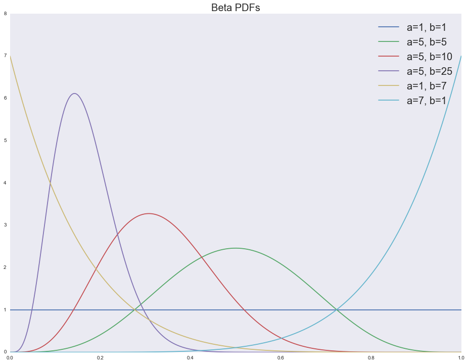

It turns out that having some prior expectations about the true value of the conversion, we can use the Bayes theorem and update our expectations when new data arrive. And the form of the prior distribution after updating the expectations remains the same beta distribution. So, we have the following model:

\begin{array}{lcr} θ_{i} & \sim & Beta (α_{i}, β_{i}) \\ y_{i} & \sim & Bernoulli (θ_{i}) \end{array}

$\large\begin{array}{lcr} \theta_i &\sim& \text{Beta}\left(\alpha_i, \beta_i\right) \\ y_i &\sim& \text{Bernoulli}\left(\theta_i\right) \end{array}$

, : ( ) ( ) , . , , , :

- $\forall i, \alpha_i = \beta_i = 1$ ;
- $\theta_i \sim \text{Beta}\left(\alpha_i, \beta_i\right)$ ;
- $k = \arg\max_{i} \theta_i$ ;
- $k$ - $y \in \left\{0, 1\right\}$ ( , );
- ( batch mode, , ):
- $\alpha_i := \alpha_i + y$
- $\beta_i := \beta_i + 1 - y$

, . Beta-Bernoulli , .. at $t \rightarrow \infty$ , , . , :

$\theta^*$ , , $\theta^*$ ; , , , ;

( -), , ;
, , , , , CTR, .

Experiment

. , , . , A/B/n-, .

 #   n_variations = 5 #     n_switches = 5 #  n_period_len      n_period_len = 2000 #       # ,   ,      ,  n_period_len p_true_periods = np.array([ [1, 2, 3, 4, 5], [2, 3, 4, 5, 1], [3, 4, 5, 2, 1], [4, 5, 3, 2, 1], [5, 4, 3, 2, 1]], dtype=np.float32).T**3 p_true_periods /= p_true_periods.sum(axis=0) #    ax = sns.heatmap(p_true_periods) ax.set(xlabel='Periods', ylabel='Variations', title='Probabilities of variations') plt.show()

: , . , n_period_len .

( ). , — ( ). , ( / — ); , . ( ), , , , . : , ( ) . . , ( , .. — ). .

 x_support = np.linspace(0, 1, 1000) alpha = dict([(i, [1]) for i in range(n_variations)]) beta = dict([(i, [1]) for i in range(n_variations)]) cmap = plt.get_cmap('jet') colors = [cmap(i) for i in np.linspace(0, 1, n_variations)] actionspp = [] for ix_period in range(p_true_periods.shape[1]): p_true = p_true_periods[:, ix_period] is_converged = False actions = [] for ix_step in range(n_period_len): theta = dict([(i, np.random.beta(alpha[i][-1], beta[i][-1])) for i in range(n_variations)]) k, theta_k = sorted(theta.items(), key=lambda t: t[1], reverse=True)[0] actions.append(k) x_k = np.random.binomial(1, p_true[k], size=1)[0] alpha[k].append(alpha[k][-1] + x_k) beta[k].append(beta[k][-1] + 1 - x_k) expected_reward = dict([(i, alpha[i][-1]/float(alpha[i][-1] + beta[i][-1])) for i in range(n_variations)]) estimated_winner = sorted(expected_reward.items(), key=lambda t: t[1], reverse=True)[0][0] print 'Winner is %i' % i actions_loc = pd.Series(actions).value_counts() print actions_loc actionspp.append(actions_loc.to_dict()) for i in range(n_variations): plt.axvline(x=p_true[i], color=colors[i], linestyle='--', alpha=0.3, label='true value of %i' % i) plt.plot(x_support, stats.beta.pdf(x_support, alpha[i][-1], beta[i][-1]), label='distribution of %i' % i, color=colors[i]) plt.legend(prop={'size': 20}) plt.title('Period %i; winner: true is %i, estimated is %i' % (ix_period, p_true.argmax(), estimated_winner), fontsize=20) plt.show() actionspp = dict(enumerate(actionspp))

 Winner is 4 4 1953 3 19 2 12 1 8 0 8 dtype: int64

 Winner is 4 3 1397 4 593 1 6 2 3 0 1 dtype: int64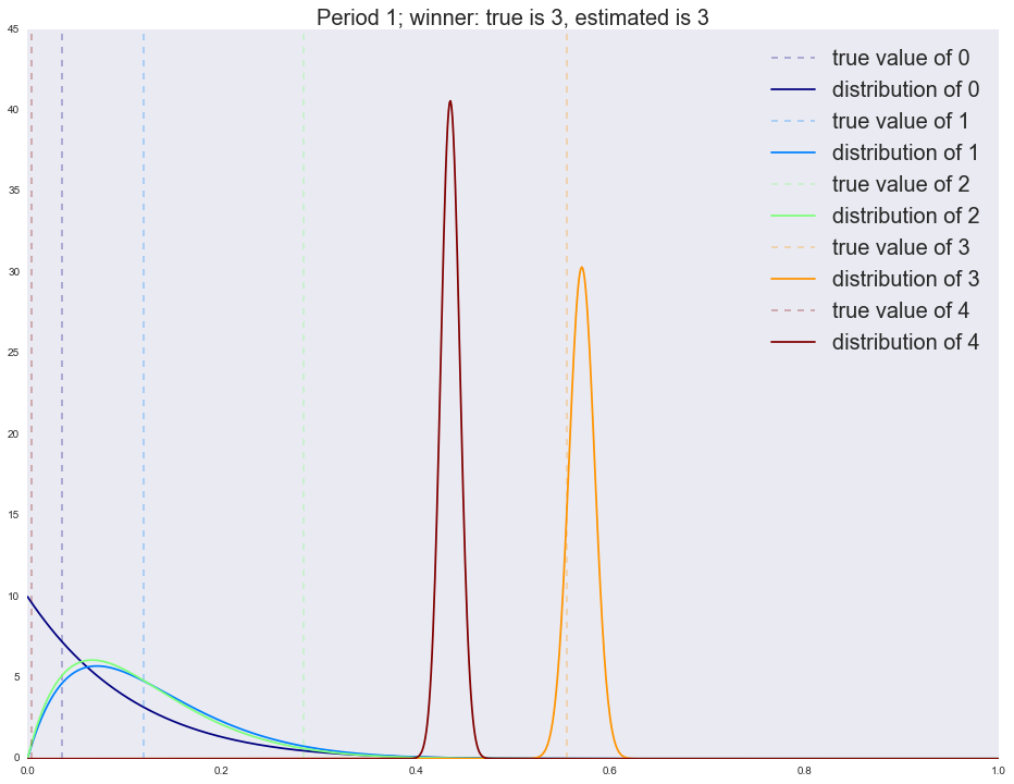

 Winner is 4 2 1064 3 675 4 255 1 3 0 3 dtype: int64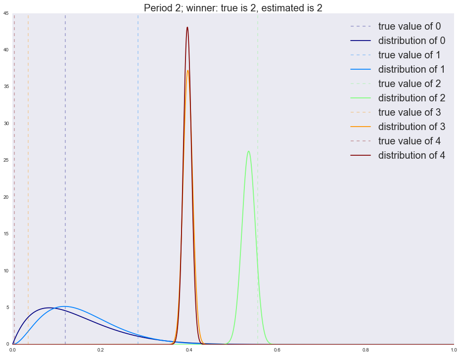

 Winner is 4 1 983 2 695 4 144 3 134 0 44 dtype: int64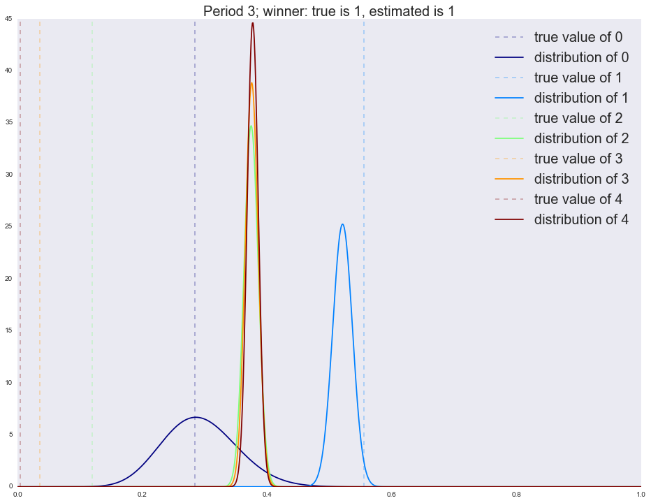

 Winner is 4 1 1109 0 888 4 2 2 1 dtype: int64

, .

 df = [] for pid in actionspp.keys(): for vid in actionspp[pid].keys(): df.append({ 'Period': pid, 'Variation': vid, 'Probapility': actionspp[pid][vid]/1000.0 }) df = pd.DataFrame(df) ax = sns.barplot(x="Period", y="Probapility", hue="Variation", data=df) ax.set(title="Ratio of traffic used for variations per period") plt.show()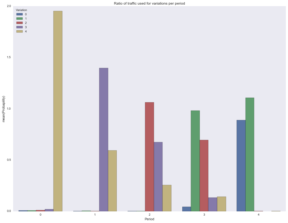

 n_period_len = 3000 alpha = dict([(i, [1]) for i in range(n_variations)]) beta = dict([(i, [1]) for i in range(n_variations)]) decay = 0.99 plot_step = 25 for f in glob.glob("./../images/mab_gif/*.png"): os.remove(f) img_ix = 0 height = 10 # 15 for ix_period in range(p_true_periods.shape[1]): p_true = p_true_periods[:, ix_period] is_converged = False actions = [] for ix_step in tqdm_notebook(range(n_period_len)): if ix_step % plot_step == 0: expected_reward = dict([(i, alpha[i][-1]/float(alpha[i][-1] + beta[i][-1])) for i in range(n_variations)]) estimated_winner = sorted(expected_reward.items(), key=lambda t: t[1], reverse=True)[0][0] fig, ax = plt.subplots() ax.set_ylim(0, height) ax.set_xlim(0, 1) for i in range(n_variations): ax.axvline(x=p_true[i], color=colors[i], linestyle='--', alpha=0.3, label='true value of %i' % i) ax.plot(x_support, stats.beta.pdf(x_support, alpha[i][-1], beta[i][-1]), label='distribution of %i' % i, color=colors[i]) ax.legend(prop={'size': 20}) ax.set_title('Period %i, step %i; winner: true is %i, estimated is %i' % (ix_period, ix_step, p_true.argmax(), estimated_winner), fontsize=20) fig.savefig('./../images/mab_gif/%i.png' % img_ix, dpi=80) img_ix += 1 plt.close(fig) theta = dict([(i, np.random.beta(alpha[i][-1], beta[i][-1])) for i in range(n_variations)]) k, theta_k = sorted(theta.items(), key=lambda t: t[1], reverse=True)[0] actions.append(k) x_k = np.random.binomial(1, p_true[k], size=1)[0] alpha[k].append(alpha[k][-1] + x_k) beta[k].append(beta[k][-1] + 1 - x_k) if decay > 0: for i in range(n_variations): if i == k: continue alpha[i].append(max(1, alpha[i][-1]*decay)) beta[i].append(max(1, beta[i][-1]*decay)) print img_ix for f in glob.glob("./../images/mab_gif/mab.gif"): os.remove(f) !convert -delay 5 $(for i in $(seq 1 1 600); do echo ./../images/mab_gif/$i.png; done) -loop 0 ./../images/mab_gif/mab.gif for f in glob.glob("./../images/mab_gif/*.png"): os.remove(f)