learnopengl. Lesson 1.8 - Coordinate Systems

In the previous lesson we learned about the benefits that can be obtained from the transformation of vertices by transformation matrices. OpenGL assumes that all the vertices that we want to see will be in normalized device coordinates after starting the shader (NDC). This means that the x, y, and z coordinates of each vertex must be between -1.0 and 1.0; coordinates outside this range will not be visible. Usually we specify the coordinates in the range that we set up on our own, and in the vertex shader we translate these coordinates into NDC. Then, these NDCs are transferred to the rasterizer to convert them to two-dimensional coordinates / pixels of your screen.

The transformation of coordinates into normalized, and then into screen coordinates is usually carried out step by step, and, before the final transformation into screen coordinates, we translate the object vertices into several coordinate systems. The advantage of converting coordinates through several intermediate coordinate systems is that some operations / calculations are easier to perform in certain systems, and this will soon become obvious. In total there are 5 different coordinate systems that are important to us:

1. Local space (or Object space)
2. World space
3. View space (or Observer)
4. Clipping space
5. Screen space

Our vertices will be transformed into all these different states before they become fragments.

Probably now you are completely confused by the fact that each space or coordinate system is of itself, so we will look at them in a more understandable form, showing the overall picture and what each of the spaces really does.

General scheme

To convert coordinates from one space to another, we will use several transformation matrices, among which, the most important are the matrices of Model , View and Projection . The coordinates of our vertices begin in local space as local coordinates , and are subsequently transformed into world coordinates , then coordinates of the form , clipping , and finally, everything ends with screen coordinates . The following image shows this sequence, and what each transformation does:

1. Local coordinates are the coordinates of your object measured relative to the reference point located where the object itself begins.
2. In the next step, the local coordinates are converted to the coordinates of the world space, which by their meaning are the coordinates of a larger world. These coordinates are measured relative to the global reference point, the same for all other objects located in world space.
3. Then we transform the world coordinates into the coordinates of the space of the View in such a way that each vertex becomes visible as if it was viewed from the camera or from the point of view of the observer.
4. After the coordinates have been converted to the view space, we want to project them into the clipping coordinates. The clipping coordinates are valid in the range of -1.0 to 1.0 and determine which vertices appear on the screen.
5. And finally, in the transformation process, which we call the transformation of the viewport ,
   we convert the clipping coordinates from -1.0 to 1.0 into the screen coordinates area specified by the glViewport function.

After all this, the resulting coordinates are sent to the rasterizer for turning them into fragments.

Probably you have already understood a little what each coordinate space is used for. The reason why we transform our vertices into these different coordinate spaces is that some operations become clearer or simpler in certain coordinate systems.

For example, the modification of your object is most reasonable to perform in local space, and the calculation of operations taking into account the location of other objects is better done in world coordinates, etc. If desired, we could define one transformation matrix that transformed the coordinates from the local space into the cut-off space in one step, but this would deprive us of flexibility.

Below we discuss each coordinate system in more detail.

Local space

Local space is a coordinate system that is local to an object, i.e. starts at the same point as the object itself. Imagine you created a cube in a simulation software package (similar to Blender). The starting point of your cube is probably located at (0,0,0), even though the cube may be located elsewhere in the application coordinates. It is possible that all the models you create have a starting point (0,0,0). Therefore, all the vertices of your model are in local space: all their coordinates are local to your object.

The vertices of the container we used were defined with coordinates between -0.5 and 0.5, with a starting point of 0.0. These are local coordinates.

World space

If we directly import all our objects into the application, they will probably be piled on top of each other near the world reference point (0.0.0), and this is not what we want. We need to determine the position of each object to place them in a wider space. Coordinates in world space, this is exactly what their name says: coordinates of all your peaks relative to the (game) world. This is the coordinate space in which you would like to see your objects transformed in such a way that they would be distributed in space (and preferably realistic). The coordinates of your object are converted from local to world space; This is done through the model matrix.

The model matrix is ​​a matrix that moves, scales and / or rotates your object for its location in world space in the position / orientation in which the object should be. Imagine this as a transformation of a building that was scaled (it was too large in the local space), moved to the suburbs, and slightly turned to the left along the Y axis in such a way that it exactly approached the neighboring houses. You can perceive the matrix from the previous lesson, in which we moved the container around the scene, as a kind of model matrix; with its help, we recalculated the local coordinates of the container to place it in different places of the scene / world.

View Space

View Space is what people commonly call an OpenGL camera (sometimes also called a camera space or an observer space ). The view space is the result of transforming world coordinates into coordinates that look as if the user is looking at them from the front. Thus, the view space is the space visible through the camera's viewfinder. This is usually achieved by a combination of such shifts and scene rotations that some objects are located in front of the camera. These combined transformations are typically stored in a view matrix , which transforms the world coordinates into a view space. In the next lesson we will widely discuss how to create such a view matrix to simulate a camera.

Clipping space

After completion of the vertex shaders, OpenGL expects that all coordinates will be in a certain range, and everything that goes beyond its boundaries will be clipped . Trimmed coordinates are discarded, and the rest become fragments visible on the screen. This is where the clipping space got its name.

Setting all visible coordinates to values ​​from the range [-1.0, 1.0] is in fact intuitively incomprehensible, so for work we define our own set of coordinates and then convert them back to NDC, as expected by OpenGL.

To convert the coordinates from the view space to the clipping space, we define a so-called projection matrix , which defines a range of coordinates, for example, from -1000 to 1000 on each axis. The projection matrix transforms the coordinates of this range into the normalized coordinates of the device (-1.0, 1.0). All coordinates outside the specified interval will not fall into the area [-1.0, 1.0], and, therefore, will be cut off. In the range that we specified by the projection matrix, the coordinate (1250, 500, 750) will not be visible, since its X component goes beyond the boundary, therefore it will be converted to a value greater than 1.0 in NDC, and therefore, the vertex will be clipped .

Please note that if outside of the cutoff volume there is not a whole primitive, for example, a triangle, but only a part of it, then OpenGL will rearrange this triangle in the form of one or several triangles that will be completely in the cutoff range.

This viewing volume , defined by the projection matrix, is called a truncated pyramid (frustum) and each coordinate that falls into this pyramid will be on the user's screen. The whole process of converting coordinates of a specific range into normalized device coordinates (NDC), which can easily be mapped to two-dimensional coordinates of the view space, is called projection , since the projection matrix projects the 3D coordinates onto simple-to-transform-in-2D normalized coordinates of the device.

As soon as the coordinates of all the vertices are transferred to the clipping space, the final operation, called perspective division , is performed. In it, we divide the x, y, and z components of the vertex position vector by the homogeneous component of the vector w. Perspective division converts the 4D coordinates of the clipping space into three-dimensional normalized coordinates of the device. This step is performed automatically after the completion of each vertex shader.

It is after this stage that the coordinates obtained (using the glViewport settings ) are mapped to the coordinates of the screen and turned into fragments.

The projection matrix that converts the view coordinates to cut-off coordinates can take two different forms, and each form defines its own particular truncated pyramid. We can create an orthographic projection or perspective matrix.

Orthographic projection

The orthographic projection matrix defines a truncated pyramid in the form of a parallelogram, which is a clipping space, where all vertices outside its volume are clipped. When creating an orthographic projection matrix, we specify the width, height, and length of the visible clipping pyramid. All coordinates that after their transformation by the projection matrix into the cut-off space fall into the volume bounded by the pyramid will not be clipped. The truncated pyramid looks a bit like a container:

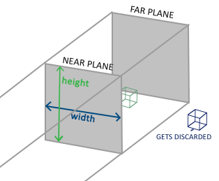
The truncated pyramid defines the region of visible coordinates and is defined by the width, height, near and far planes. Any coordinate located in front of the near plane is clipped, just as it does with the coordinates behind the rear plane. The orthographic truncated pyramid directly translates the coordinates falling into it into the normalized coordinates of the device, and the w-components of the vectors are not used; if the w-component is 1.0, then the perspective division will not change the coordinate values.

To create an orthographic projection matrix, we use the built-in function of the GLM library, called glm :: ortho :

glm::ortho(0.0f, 800.0f, 0.0f, 600.0f, 0.1f, 100.0f ); 

The first two parameters define the left and right coordinates of the truncated pyramid, and the third and fourth parameters define the lower and upper boundaries of the pyramid. These four points set the dimensions of the near and far planes, and the 5th and 6th parameters indicate the distance between them. This special projection matrix converts all coordinates that fall within the ranges of x, y and z values ​​into normalized coordinates of the device.

The orthographic projection matrix maps the coordinates directly onto a two-dimensional plane, which is your display, but in reality, direct projection gives unrealistic results because it does not take perspective into account. This corrects the perspective projection matrix.

Perspective Projection

If you have ever watched the real world , you probably noticed that objects further away look much smaller. This strange effect we call perspective . The perspective is especially noticeable when you look at the end of an endless highway or railway, as seen in the following image:

As you can see, because of the perspective it seems that the lines converge the more, the further they are. This is exactly the effect that the perspective projection tries to imitate, and it is achieved through the perspective projection matrix . The projection matrix displays the specified range of the truncated pyramid into the clipping space, and at the same time manipulates the w-component of each vertex in such a way that the farther the vertex is from the observer, the more this w-value becomes. After converting the coordinates to the clipping space, they all fall in the range from -w to w (vertices that are outside this range are truncated). OpenGL requires the final output of the vertex shader to be between -1.0 and 1.0. Thus, when the coordinates are in the cut-off space, the perspective division is applied to them:

Each component of the vertex coordinate is divided into its w-component, which reduces the coordinate values ​​in proportion to the distance from the viewer. This is another reason why the w-component is important because it helps us with a perspective projection. The coordinates obtained after this are in the normalized device space. If you are interested in understanding how orthogonal and perspective projection matrices are calculated (and you are not too afraid of mathematics), then I can recommend this excellent Songho article .

You can create a perspective projection matrix in the GLM library as follows:

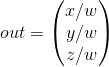
 glm::mat4 proj = glm::perspective( 45.0f, (float)width/(float)height, 0.1f, 100.0f); 

glm :: perspective creates a truncated pyramid that defines the visible space, and anything that is outside of it and will not fall into the amount of clipping space will be clipped. The perspective truncated pyramid can be represented as a trapezoidal box, each coordinate inside of which will be mapped to a point in the clipping space. An image of a perspective truncated pyramid is shown below:

The first parameter sets the value of fov (field of view), which means " field of view ", and determines how large the visible area is. For a realistic view, this parameter is usually set to 45.0f, but to get a similarity to the doom-style, you can set large values. The second parameter sets the aspect ratio, which is calculated by dividing the width of the viewing area by its height. The third and fourth parameters define the near and far plane of the truncated pyramid. Usually we set the nearest distance to 0.1f, and the farthest 100.0f. All vertices located between the near and far plane and falling into the volume of the truncated pyramid will be visualized.

If in the projection matrix the distance to the near plane is set too large (for example, 10.0f), then OpenGL cuts off all coordinates located near the camera (between 0.0 and 10.0f), which gives a visual effect familiar to video games when you can see through some objects if you get too close to them.

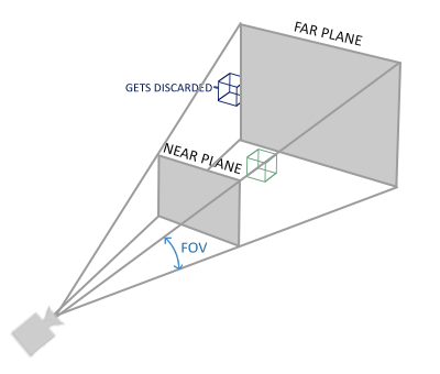
When using an orthogonal projection, each coordinate of the vertex is directly mapped to the clipping space without any imaginary perspective division (perspective division is performed, but the w-component does not affect the result (it remains equal to 1) and, therefore, has no effect). Since the orthographic projection does not take into account the perspective, the objects located further do not seem smaller, which creates a strange visual impression. For this reason, orthographic projection is mainly used for 2D rendering and various architectural or engineering applications, where we would prefer no distortion due to perspective. In applications like Blender for 3D modeling, orthographic projection is sometimes used during modeling, because it more accurately reflects the dimensions and proportions of each object. The following is a comparison of both projection methods in Blender:

You can see that with the perspective projection, the remote vertices are much farther away, while in the orthographic projection the vertex removal rate is the same and does not depend on the distance to the observer.

Putting it all together

Create a transformation matrix for each of the above steps: model, view and projection matrix. The vertex coordinate is converted to the coordinates of the clipping space as follows:

Note that the matrix multiplication order is inverse (remember that matrix multiplication should be read from right to left). The resulting coordinate of the vertex must be assigned in the vertex shader of the built-in variable gl_Position , after which OpenGL automatically performs the promising division and clipping.

What then?
The coordinates of the vertex shader output must be in the clipping space, which we have just achieved using transformation matrices. OpenGL performs a perspective division of the coordinates of the clipping space to convert them into normalized device coordinates.
OpenGL then uses the parameters from glViewPort to map the normalized coordinates of the device to screen coordinates, in which each coordinate corresponds to a point on your screen (in our case, the area is 800x600). This process is called viewport conversion .

This topic is difficult to understand, so if you are still not quite sure about what each space is used for, then you need not worry.
')
Below you will see how we can effectively apply these coordinate spaces, and there will be enough examples in the following lessons.

Go to 3D

Now that we know how to transform the 3D coordinates into 2D coordinates, we can begin to display our objects as real 3D objects, and not as damaging 2D planes that we have shown so far.

To start drawing in 3D, we first create a matrix model. The matrix of the model consists of shifts, scaling and / or turns, which we would like to apply to transform all the vertices of the object into the global world space. Let's change our plane a bit, turning it along the X axis so that it looks like it is lying on the floor. The matrix of the model will look as follows:

 glm::mat4 model; model = glm::rotate(model, -55.0f, glm::vec3(1.0f, 0.0f, 0.0f); 

Multiplying the coordinates of the vertices by this matrix of the model, we transform them into world coordinates. Our plane lying on the floor is thus a plane in world space.

Then we need to create a view matrix. In order for the object to become visible, we need to move a little back in the scene (because the observer's point of view in world space is at the origin (0,0,0)). To move around the scene, think about the following:

Moving the camera back is the same as moving the whole scene forward.

This is exactly what the view matrix does: we move the entire scene to the opposite side of the one into which we would like to move the camera. Since we need to move backwards, and since OpenGL uses the right coordinate system, we must move in the positive z direction. We do this by shifting the entire scene to the negative side of the z axis. This gives the impression that we are moving backwards.

Right Coordinate System

By convention, OpenGL is the right coordinate system. This basically means that the positive X axis is pointing to the right from you, the positive Y axis is up, and the positive Z axis is on you (that is, back). Imagine that your screen is the center of three axes, and the positive Z axis passes through the screen towards you. Axes are depicted as follows:

To understand why this system is called right, do the following:

• Stretch your right hand up along the positive Y axis.
• Let your thumb point to the right.
• Let the index finger point upwards.
• Now bend your middle finger 90 degrees.

If you did everything correctly, your thumb should indicate the direction of the positive X axis, the index finger the positive Y axis, and the middle finger on the positive z axis. If you do the same with your left hand, you will see that the Z axis changes direction. This coordinate system is known as the left and is commonly used in DirectX. Note that in the normalized coordinates of the device, OpenGL actually uses the left system (the projection matrix switches directions).

We will discuss moving around the scene in more detail in the next lesson. At the moment, the view matrix looks like this:

 glm::mat4 view; //  ,        ,      view = glm::translate(view, glm::vec3(0.0f, 0.0f, -3.0f)); 

The last thing we need to determine is the projection matrix. For our scene we will use a perspective projection, so we will declare the matrix as follows:

 glm::mat4 projection; projection = glm::perspective(45.0f, screenWidth / screenHeight, 0.1f, 100.0f); 

Be careful when specifying degrees in GLM. Here we set the fov parameter to 45 degrees, but some GLM implementations accept fov in radians, in which case you need to set it as glm :: radians (45.0).

Now that we have created the transformation matrices, we must transfer them to our shaders. First, let's declare the uniform matrix in the vertex shader of the transformation matrix and multiply them by the vertex coordinates:

 #version 330 core layout (location = 0) in vec3 position; ... uniform mat4 model; uniform mat4 view; uniform mat4 projection; void main() { // ,       gl_Position = projection * view * model * vec4(position, 1.0f); ... } 

We also need to send the matrices to the shader (this is usually done for each iteration, since the transformation matrices tend to change often):

 GLint modelLoc = glGetUniformLocation(ourShader.Program, "model"); glUniformMatrix4fv(modelLoc, 1, GL_FALSE, glm::value_ptr(model)); ... //        

Now that our vertex coordinates are transformed by the matrices of the model, the view and the projection matrix, the final object should:

• Rejected back to the floor.
• A little removed from us.
• To be displayed taking into account the perspective (its dimensions should become smaller with increasing distance to the viewer).

Let's check if the result really meets these requirements:

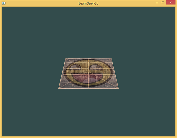
It really looks like a 3D plane that rests on some imaginary floor. If you didn’t get the same result, check out the full source code , the vertex shader, and the fragment shader .

More 3D

So far we have been working with the 2D plane, but in 3D space, so let's take a little adventure and expand our 2D plane to a 3D cube.

To display the cube, we need a total of 36 vertices (6 sides * 2 triangles * 3 vertices each). To score 36 vertices is quite a lot, so you can take them here . Please note that to get the resulting color of the fragments, we will use only the texture, so we skip the color values ​​of the vertices.

Removing color attributes from a vertex array changes the size of the “step” between the vertices, so you need to correct this parameter in the calls to the glVertexAttribPointer function:

 // Position attribute glVertexAttribPointer(0, 3, GL_FLOAT, GL_FALSE, 5 * sizeof(GLfloat), (GLvoid*)0); ... // TexCoord attribute glVertexAttribPointer(2, 2, GL_FLOAT, GL_FALSE, 5 * sizeof(GLfloat), (GLvoid*)(3 * sizeof(GLfloat))); 

For a change, let's set the cube rotation:

 model = glm::rotate(model, (GLfloat)glfwGetTime() * 50.0f, glm::vec3(0.5f, 1.0f, 0.0f)); 

And now draw a cube using glDrawArrays, but this time with the number of 36 vertices.

 glDrawArrays(GL_TRIANGLES, 0, 36); 

You should get something like this:

The object is a bit like a cube, but something is wrong with it. Some sides of the cube are drawn on top of its other sides. This is because when OpenGL renders your cube triangle-behind-triangle, it overwrites the pixels in the frame buffer, despite its contents and what has already been drawn in it before. Because of this, some triangles are drawn one on top of the other, although they should not overlap each other.

Fortunately, OpenGL stores depth information in a buffer called Z-Buffer , which allows OpenGL to decide when to draw on top of a pixel and when not. With the Z-buffer, we can configure OpenGL to do a pixel depth check.

Z-buffer

OpenGL stores all depth information in a Z-buffer, also known as a depth buffer . GLFW creates this buffer automatically (it also has a frame buffer that stores the colors of the output image). The depth is stored for each fragment (as a z-value) and whenever the fragment displays its color, OpenGL compares its depth value with the values ​​from the Z-buffer, and if the current fragment is behind the other fragment, it is discarded, otherwise it is overwritten. . This process is called depth checking and is performed automatically by OpenGL.

However, if we want to be sure that OpenGL does perform depth checking, we first need to turn it on, because it is turned off by default. Depth checking is enabled using the glEnable function. The glEnable and glDisable functions allow you to enable / disable certain OpenGL features. OpenGL options are enabled / disabled until another function call is made to disable / enable them. At this point, we want to enable depth checking, including the GL_DEPTH_TEST parameter:

 glEnable(GL_DEPTH_TEST); 

Since we use the depth buffer, we need to clear it before each iteration of the visualization (otherwise the buffer will contain information about the depth of previous frames). We can clear the depth buffer in the same way as the color buffer, by specifying the GL_DEPTH_BUFFER_BIT bit in the glClear function:

 glClear(GL_COLOR_BUFFER_BIT | GL_DEPTH_BUFFER_BIT); 

Let's rerun our program and see if OpenGL now performs a depth check:

That's all! Our cube is fully textured, with the correct depth checking, and also rotates. Here is the source code for verification.

More cubes!

Suppose we would like to display 10 of our cubes on the screen. All cubes look the same, but will differ in location in world space and angle of rotation. The graphical representation of the cube is already defined, and in order to draw a few more objects, we no longer need to change the buffers or attribute arrays. The only thing we need to fix for each object is its model matrix, thanks to which we transform the local coordinates of the cube into world ones.

First, let's define for each cube a displacement vector that will set the position of an object in world space. We write 10 positions of cubes in the array glm :: vec3:

 glm::vec3 cubePositions[] = { glm::vec3( 0.0f, 0.0f, 0.0f), glm::vec3( 2.0f, 5.0f, -15.0f), glm::vec3(-1.5f, -2.2f, -2.5f), glm::vec3(-3.8f, -2.0f, -12.3f), glm::vec3( 2.4f, -0.4f, -3.5f), glm::vec3(-1.7f, 3.0f, -7.5f), glm::vec3( 1.3f, -2.0f, -2.5f), glm::vec3( 1.5f, 2.0f, -2.5f), glm::vec3( 1.5f, 0.2f, -1.5f), glm::vec3(-1.3f, 1.0f, -1.5f) }; 

Now, within the game cycle, we are going to call the function glDrawArrays 10 times, but at the same time, before each visualization, we will transfer different matrixes of the model to the vertex shader. We will create another small loop inside the game loop, which will draw our object 10 times with different values ​​of the model matrix. Note that for each container we also added a slight rotation.

 glBindVertexArray(VAO); for(GLuint i = 0; i < 10; i++) { glm::mat4 model; model = glm::translate(model, cubePositions[i]); GLfloat angle = 20.0f * i; model = glm::rotate(model, angle, glm::vec3(1.0f, 0.3f, 0.5f)); glUniformMatrix4fv(modelLoc, 1, GL_FALSE, glm::value_ptr(model)); glDrawArrays(GL_TRIANGLES, 0, 36); } glBindVertexArray(0); 

This code fragment will update the model matrix with each image of a new cube, and will do it all in all 10 times. Now we need to see the world filled with ten arbitrarily turned cubes:

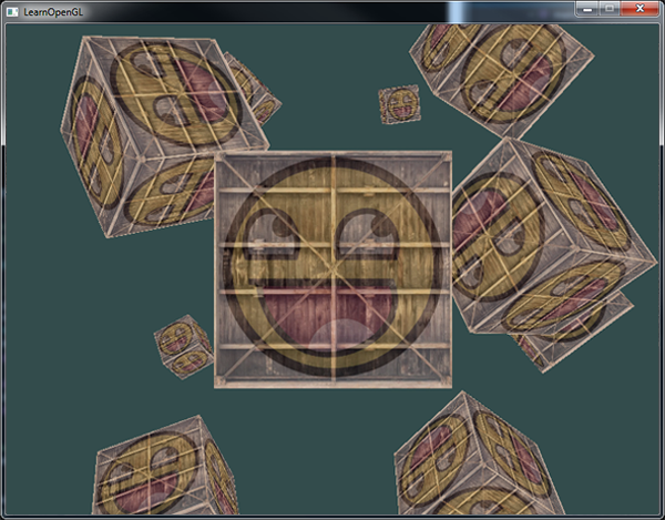
Fine! Looks like our container found some friends like it. If you are stuck, before continuing to look at what could be the problem and compare your code with the source code , vertex and fragment shader.

Exercises

• When creating a projection matrix, try experimenting in the GLM projection function with FOV parameters and an aspect ratio .
  See if you can figure out how these parameters affect the perspective truncated pyramid.
• Play around with the view matrix, shifting the coordinates in different directions and see how the scene changes. Think of the view matrix as a camera.
• Try to rotate every third container (including 1), and leave the rest stationary, using only the model matrix:
  the decision .