Cook ML Boot Camp III: Starter Kit
March 16 ended the machine learning competition ML Boot Camp III . I am not a real welder, but, nevertheless, I was able to achieve the 7th place in the final results table. In this article I would like to share how to start participating in such kind of championships, what you should pay attention to for the first time when solving a problem, and tell about your approach.
ML Boot Camp III
This is an open machine learning championship organized by the Mail.Ru Group. As a task, it was proposed to predict whether the player will remain in the online game or leave it. As data, the organizers gave already processed statistics on users for the last 2 weeks.
- maxPlayerLevel - the maximum level of the game that the player has passed;
- numberOfAttemptedLevels - the number of levels that the player tried to pass;
- attemptsOnTheHighestLevel - the number of attempts made at the highest level;
- totalNumOfAttempts - total number of attempts;
- averageNumOfTurnsPerCompletedLevel - the average number of moves performed on successfully completed levels;
- doReturnOnLowerLevels - whether the player made returns to the game at levels already completed;
- numberOfBoostersUsed - the number of boosters used;
- fractionOfUsefullBoosters - the number of boosters used during successful attempts (the player has passed the level);
- totalScore - total points scored;
- totalBonusScore - total bonus points earned;
- totalStarsCount - the total number of stars scored;
- numberOfDaysActuallyPlayed - the number of days the user played the game.
More details about the championship can be found on the project website .
Read the rules
In contrast to the instructions for household appliances, there is useful information. What to look for:
- input and output formats;
- maximum number of packages per day;
- quality criterion / evaluation function.
The latter is perhaps the most important part of the rules, since it is precisely this function that we will need to minimize (sometimes maximize). This time the logarithmic loss function was used:
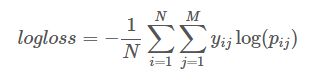
Here
N is the number of examples.
M is the number of classes (there are only two)
Pij is the predicted probability of class i belonging to example i
Yij - equals 1 if example i really belongs to class j, and 0 otherwise
It is important to note that this formula strongly “punishes” self-confidence in the answers. Therefore, as a solution, it is more profitable to send the probability that the player will continue to play instead of the unambiguous "1" and "0".
Sometimes studying the evaluation function allows you to cheat a little and get extra points (as the winner of the past and the current competition did ).
More information on different metrics can be read here .
Tools

There are many tools that can be used during the championship. If the conversations of people about machine learning sound like curses to you, I can advise you to gallop around ML and familiarize yourself with the basic algorithms here .
This time most of the participants chose between Python and R. The general recommendation is: stick to one language and explore the possibilities of the available tools more deeply. For both languages there are good solutions, and the most popular libraries (for example XGBoost) are available both there and there.
In the case of urgent need, you can always do some separate calculation using a different package. For example, the t-SNE transform, which in the python implementation drops helplessly, eating up all the memory.
I chose python, and my final solution used the following libraries:
- scikit learn is a great toolkit for machine learning. Initially, you can only be limited to her.
- XGBoost - gradient boosting. One of the most favorite libraries of participants in machine learning championships.
- LightGBM is an alternative to XGBoost, in my case it worked an order of magnitude faster than the latter, but produced slightly less accurate results.
- Lasagne is a library for creating and training neural networks using Theano. As an alternative, you can try Keras - it looks a little more simple and there is more documentation on it. But the horses at the crossing do not change and I decided to stick with the initial choice.
First submit
To begin with, let's try to read all the input data and display a test answer consisting of only zeros.
>>> import numpy as np >>> import pandas as pd >>> X_train = pd.read_csv('x_train.csv', sep=';') >>> X_test = pd.read_csv('x_test.csv', sep=';') >>> y_train = pd.read_csv('y_train.csv', header=None).values.ravel() >>> print(X_train.shape, X_test.shape, y_train.shape) (25289, 12) (25289, 12) (25289,) >>> result = np.zeros((X_test.shape[0])) >>> pd.DataFrame(result).to_csv('submit.csv', index=False, header=False) After you have checked the load / save data and obtained a point of reference for evaluation, you can train a simple model. As an example, I took RandomForestClassifier.
>>> from sklearn.ensemble import RandomForestClassifier >>> clf = RandomForestClassifier() >>> clf.fit(X_train, y_train) >>> result = clf.predict_proba(X_test)[:,1] >>> pd.DataFrame(result).to_csv('submit.csv', index=False, header=False) If we run the previous example again and send the result for verification, then, with a high probability, we will get another assessment. This is due to the fact that within many algorithms a random number generator is used. This behavior greatly complicates the assessment of the impact of future changes in the model on the final result. To avoid this problem, we can:
>>> np.random.seed(2707) >>> clf = RandomForestClassifier(random_state=2707) ... or
>>> runs = 1000 >>> results = np.zeros((runs, X_test.shape[0])) >>> for i in range(runs): … clf = RandomForestClassifier(random_state=2707+i) … clf.fit(X_train, y_train) … results[i, :]=clf.predict_proba(X_test)[:,1] >>> result = results.mean(axis=0) In the second variant, we get a more stable result, but it is obvious that it takes much more time to calculate, so I used it already for the final checks.
More examples can be found in the training article from the organizers. There you can also find information about working with categorical features, which I do not touch on in this article.
Data preparation

In order to lower the threshold of entry, the organizers prepared the data fairly well, and no further cleaning was required. Moreover, attempts to remove duplicates or outliers in a training set only led to a deterioration in the result.
About duplicates, it is worth noting that they often belonged to different classes (users with the same data could either stay or leave the game), and without additional information, it is difficult to make an accurate prediction. Fortunately, most models coped with this on their own, deriving probabilities that minimize the estimated function, in our case, log loss.
UPD: the participant from third place still managed to use this fact to his advantage.
The data prepared by the organizers is rather an exception to the rules, which means you need to be ready to process them yourself. In addition to duplicate rows and outliers, the data may contain missing values. It is too wasteful to delete lines with missing values, since they still contain useful information. Therefore, we have 2 options left:
- leave everything as it is: some algorithms can work with missing (NA) values;
- try to restore them.
To restore, you can simply replace with the more common (categorical signs), average or median value. In python, you can use the sklearn.preprocessing.Imputer class for this. There are more complex methods using other features (for example, the average value among users of the same level), I even tried to train another model that predicts the missing value for other columns. Oh yeah, I wrote above that the data is prepared and there are no missing values, in fact this is not quite so.
If you read the rules carefully, it becomes clear that almost all signs are statistics based on logs for 2 weeks. A more detailed study of the data shows that quite a few users started playing earlier than 2 weeks ago. If we screen them out, then I received incredibly good marks for cross-validation, which led me to believe that improving predictions for the remaining “dirty” data might be the key to victory. Attempts to restore data to the user at the time of 2 weeks ago did not give a strong increase, but I left this decision and later used it together with others.
Another trick that came to my mind is to multiply the number of signs of such users by -1. This separates them from the rest of the mass in training and shows itself well, especially considering the simplicity of the method.
All data: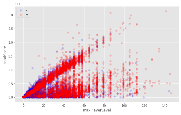
Only users who started playing during the 2-week period:
Attempt to recover data in other columns: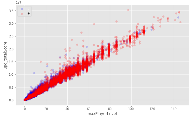
“Invert” for users who started playing earlier than 2 weeks ago:
In certain cases, it makes sense to immediately get rid of some signs:
- constant signs;
- two strongly correlated traits (only one of them is needed);
- signs with close to zero variance.
Although this increases the speed of calculations, and sometimes improves the overall quality of models, but with the removal of signs, you need to be extremely careful.
The last thing you can do with the initial data is scaling. By itself, it does not change the dependencies between features, but it can significantly improve the predictions for some (for example, linear) models. In python, you can use the following classes: sklearn.preprocessing.StandardScaler , sklearn.preprocessing.MinMaxScaler and sklearn.preprocessing.MaxAbsScaler .
Each of the data transformations should be carefully checked. What works in one case can have a negative effect in another, and vice versa.
Always (!) Check that the test sample passes through the exact same transformations as the training one.
We check ourselves
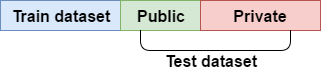
The entire data set is divided into two parts: the training and test samples. The test sample is divided in a 40/60 ratio into public and hidden. How well the model predicted the result for the public part determines the position in the leaderboard throughout the championship, and the prediction score for the hidden part becomes available only at the very end and determines the final positions of the participants.
If we focus only on the results of the public part of the test sample, then this will most likely lead to a retraining of the model and a strong drop in the rating after the discovery of hidden results. To avoid this, as well as to be able to locally check how much the model has improved / deteriorated, cross-validation is used.

We break the data into K-folds: we fold the K-1 folds, and for the rest we predict and consider the prediction estimate. So repeat for all K folds. The final score is calculated as the average of the scores for each fold.
In addition to the average value, you should pay attention to the standard deviation of the estimates (std), this parameter may be even more important than the average fold score, since Shows how strong the spread in the predictions for different folds. The value of std can grow strongly with increasing K, you should bear this in mind and not be afraid.
An important role is played by the quality of splitting into folds. To preserve the distribution of classes at the breakdown, I used sklearn.model_selection.StratifiedKFold . This is especially important if the classes are initially highly unbalanced. In addition, there may be other problems with the distribution of data on the folds (days of the week, time, users, etc.) that need to be checked and corrected separately.
As before, wherever a random number generator is used, we fix the seed value so that any result can be reproduced.
>>> from sklearn.model_selection import StratifiedKFold, cross_val_score >>> clf = RandomForestClassifier(random_state=2707) >>> kf = StratifiedKFold(random_state=2707, n_splits=5, shuffle=True) >>> scores = cross_val_score(clf, X_train, y_train, cv=kf) >>> print("CV scores:", scores) CV scores: [ 0.8082625 0.81059707 0.8024911 0.81431679 0.81926043] >>> print("mean:", np.mean(scores)) mean: 0.810985579862 >>> print("std:", np.std(scores)) std: 0.00564433052781 Using different schemes for cross-validation, it is desirable to achieve a minimum difference of local and public assessment. If the estimates do not coincide and local cross-validation is considered correct, it is customary to rely on a local assessment.
Complicate the model (what works is not ugly)
Tuning
The selection of hyper-parameters for MO algorithms can be considered as the task of minimizing a function that returns an estimate of the model with these parameters for cross-validation.
Consider several options for solving this problem.
- Bruteforce ( sklearn.model_selection.GridSearchCV ). Despite brute force, this method can be quite effective. XGBoost models I tuned them. And here is a good guide how you can do it and not wait a few days. The method is also good because in order to save time, it makes you better understand the value of hyper-parameters.
- Randomized bust ( sklearn.model_selection.RandomizedSearchCV ). As an advantage, it can be noted that the number of rebounds can be set regardless of the number of parameters.
- hyperopt . It allows you to select many hyper-parameters at once, including for neural networks with different number of layers, which is especially convenient if you need to find a configuration from which you will then push off.
- Differential evolution .
- Manual fit, etc.
By the way, if for cross-validation you use the cros_val_score Learn library cros_val_score method, then you should pay attention to the fact that some algorithms can take into their fit method a metric that they will minimize when training. And in order to set this parameter during cross-validation, you need to use fit_params .
The UPD: eval_metric parameter in the xgboost and LightGBM libraries sets the metric by which eval_set is evaluated for early stopping. In other words, in the fit method, the data set is transferred, on which the model is evaluated using eval_metric at each step of the gradient boosting, in the case where the early_stopping_rounds steps in a row the assessment for eval_set does not improve, then the learning stops.
clf = xgb.XGBClassifier(seed=2707) kf = StratifiedKFold(random_state=2707, n_splits=5, shuffle=True) scores = cross_val_score(clf, X_train, y_train, cv=kf, scoring='neg_log_loss', fit_params={'eval_metric':'logloss'}) Calibration (Hello Garus!)
The idea of calibration is that if the model gives a prediction of belonging to the class of 0.6, then among all the samples to which she gave this prediction, 60% really belong to this class. The Scikit Learn library contains the sklearn.calibration.CalibratedClassifierCV class for this. This can improve the assessment, but we must remember that the calibration mechanism is used for cross-validation, which means that it will greatly increase the training time.
from sklearn.ensemble import RandomForestClassifier from sklearn.calibration import CalibratedClassifierCV kf = StratifiedKFold(random_state=2707, n_splits=5, shuffle=True) clf = RandomForestClassifier(random_state=2707) scores = cross_val_score(clf, X_train, y_train, cv=kf, scoring="neg_log_loss") print("CV scores:", -scores) print("mean:", -np.mean(scores)) clf = CalibratedClassifierCV(clf,method='sigmoid', cv=StratifiedKFold(random_state=42, n_splits=5, shuffle=True)) scores = cross_val_score(clf, X_train, y_train, cv=kf, scoring="neg_log_loss") print("CV scores:", -scores) print("mean:", -np.mean(scores)) CV scores: [ 1.12679227 1.01914874 1.24362513 0.97109882 1.07280166] mean: 1.08669332288 CV scores: [ 0.41028741 0.4055759 0.4134125 0.40244068 0.39892905] mean: 0.406129108769 <--- Bagging
The idea is to run the same algorithm on different (not complete) sets of training samples and traits and then use the average prediction of such models. As always, Scikit Learn already contains everything that we need, which greatly saves our time, just use the sklearn.ensemble.BaggingClassifier class.
from sklearn.ensemble import RandomForestClassifier, BaggingClassifier kf = StratifiedKFold(random_state=2707, n_splits=5, shuffle=True) clf = RandomForestClassifier(random_state=2707) scores = cross_val_score(clf, X_train, y_train, cv=kf, scoring="neg_log_loss") print("CV scores:", -scores) print("mean:", -np.mean(scores)) clf = BaggingClassifier(clf, random_state=42) scores = cross_val_score(clf, X_train, y_train, cv=kf, scoring="neg_log_loss") print("CV scores:", -scores) print("mean:", -np.mean(scores)) CV scores: [ 1.12679227 1.01914874 1.24362513 0.97109882 1.07280166] mean: 1.08669332288 CV scores: [ 0.51778172 0.46840953 0.52678512 0.5137191 0.52285478] mean: 0.509910050424 Of course, no one forbids using it in conjunction with calibration.
Composite models
It is not uncommon for data to be divided into groups for which it is more advantageous to predict using different models. For example, some participants divided into different groups by player level and predicted them by different models.
My best model used such a principle. I divided into two groups: those who started playing within 2 weeks, and those who started earlier. And in the first group I added also those who at the time of the beginning of logging were of the 1st level, since this improved the overall rating. As models, I took xgboost with different hyper-parameters and used for them different sets of features. And when teaching the second model, I used all the data, but for users who started playing earlier than 2 weeks ago, I gave a weight equal to 3.
Dirty tricks
It should be understood that the competition and the actual use of machine learning algorithms are completely different things. Here you can make huge and slow models, which at the expense of extra days of calculations will give a fraction of percent accuracy in the assessment, or even use the manual adjustment of the answers to increase accuracy. Most importantly, beware of retraining in a public assessment.
More data!

In order to squeeze the last drops of information from the data provided to us, you can (need!) Try to generate new signs. Creating a good feature set from the data provided is often a key factor in winning machine learning championships.
- Multiplying or dividing existing features is a simple but effective way.
- Extraction of new signs. For example, the day of the week from the date, the number of characters from the text, etc.
- Nonlinear transformation of an existing trait allows one to bring the distribution of magnitude closer to normal, which in some cases (the same neural networks) gives the best result. Examples: log (x), log (x + 1), sqrt (x), sqrt (x + 1), etc.
- Other. All that you have enough imagination: the maximum degree of two, which is divided into a number, the difference in age with the president, etc. One of the signs I generated, which was used in the final models, was calculated by the formula:
raw_data['totalScore'] / (1 + np.log(1+raw_data['maxPlayerLevel']) * raw_data['maxPlayerLevel']) Now, when we have a lot of new signs, we need to somehow select the optimal set, which gives the best estimate.
Using PCA or TruncatedSVD, you can reduce the dimension of the attribute space to increase the speed of the algorithms. However, there is a big risk of ignoring non-linear dependencies between the data, as well as losing important signs completely.
Many algorithms, such as, for example, gradient boosting, due to their device make it quite easy to obtain information about the importance of a particular feature in a trained model. This information can be used to filter out unimportant columns.
import matplotlib.pyplot as plt import xgboost as xgb from xgboost import plot_importance clf = xgb.XGBClassifier(seed=2707) clf.fit(X_train, y_train, eval_metric='logloss') for a, b in sorted(zip(clf.feature_importances_, X_train.columns)): print(a,b, sep='\t\t') plot_importance(clf) plt.show() 0.014771 numberOfAttemptedLevels 0.014771 totalStarsCount 0.0221566 totalBonusScore 0.0295421 doReturnOnLowerLevels 0.0354505 fractionOfUsefullBoosters 0.0531758 attemptsOnTheHighestLevel 0.0886263 numberOfBoostersUsed 0.118168 totalScore 0.128508 averageNumOfTurnsPerCompletedLevel 0.144756 maxPlayerLevel 0.172821 numberOfDaysActuallyPlayed 0.177253 totalNumOfAttempts 
As always, you need to be extremely careful with the removal of signs. Removing unimportant signs can spoil the accuracy of prediction, and removing the most important ones, on the contrary, can improve. I used this method to screen out completely hopeless signs.
There are more classical approaches for the selection of signs. In this competition, I intensively used the greedy algorithm, the idea of which is to add new features one by one to the set and choose the one that gives the best estimate for cross-validation. You can also throw away signs one by one. Alternating these approaches, I scored the final samples. This is an easy-to-write algorithm, but it ignores features that increase accuracy well in a set with several others. From this point of view, it would be more productive to encode the use of signs by a binary vector and use a genetic algorithm.
Bug work

Glory and prizes are nice, of course, but my main motivation this time was to gain experience and knowledge. And, of course, the learning process is not without errors. Analysis of which brought me the most understanding of what I was doing. And if you are a newbie like me, then my advice is: try everything. Having several different results, it is easier to evaluate each of them relative to the others, to compare them with each other. And attempts to explain to ourselves why what is happening, lead to a deeper understanding of the operation of algorithms.
The process of working with data and models described above in the article is not linear, and during the championship I occasionally returned to new models, now to generate new features and tuning models for them. As a result, several good models have accumulated, the results of which I used for the final prediction.
In case you are stuck at dead center:
- remember the local minimum: perhaps, some idea will first give a result worse than the current one, but its further development or combination with other ideas will be your “killer feature”;
- one can almost always find scientific papers on the subject of the assignment, which may give rise to thoughts;
- study the decisions of participants of other championships (kaggle);
- Try different models or even more feature generation.
More models!

Suppose, after many agonies and sleepless nights, we got one good model with a good rating on a local CV and, ideally, a good rating in public. In addition, it turned out a couple more models of slightly worse quality. Do not immediately throw the last. The fact is that the predictions of several models can be combined in different ways and get even more accurate. This is a pretty big topic and I recommend starting with this article . Here I will share two methods of different complexity that I managed to bring to mind.
The simplest approach, and in my case also a more efficient one, turned out to be a banal arithmetic average between solutions of several models. As variations of this method, you can use the geometric mean, as well as add weight to the models.
The second approach is stacking. Here you can eat oats ... The idea is simple: use the predictions of the first level models as input to another algorithm. Sometimes initial data is added to these predictions or the results of first-level models are used to generate new features. , ( -), . : holdout set out-of-fold predictions.
Holdout set — (~10%) , , . , .
OOF predictions — K , K-1 . . : , (Variant ), , -1 , (Variant A).

def get_oof(clf): oof_train = np.zeros((X_train.shape[0],)) oof_test = np.zeros((X_test.shape[0],)) oof_test_skf = np.empty((NFOLDS, X_test.shape[0])) for i, (train_index, test_index) in enumerate(kf.split(X_train, y_train)): x_tr = X_train[train_index] y_tr = y_train[train_index] x_te = X_train[test_index] clf.train(x_tr, y_tr) oof_train[test_index] = clf.predict_proba(x_te)[:, 1] oof_test_skf[i, :] = clf.predict_proba(X_test)[:, 1] oof_test[:] = oof_test_skf.mean(axis=0) return oof_train.reshape(-1, 1), oof_test.reshape(-1, 1) ? , (data leak), , . , , , .
1: OOF predictions -.
2: K~=10, 1 holdout set.
, , . -, , , .
Don't Repeat Yourself

, . . , / , -, OOF , - .. , , , . , , .
, , . .
Results
. telegram . , 6 8 .

GitHub .
, , , .
, .
')
Source: https://habr.com/ru/post/324924/
All Articles