The winning decision of the ML Boot Camp III contest
Good day! In this article, I would like to briefly tell you about the solution that brought me the first place in the ML Boot Camp III machine learning competition from mail.ru.
I introduce myself, my name is Karachun Mikhail, I am also the winner of the previous contest mail.ru. My past decision is described here and sometimes I will refer to it.
The participants of the competition were asked to predict the probability that the player who played the online game would leave it on the basis of a sample of data. The sample contained some data on the activity of the players for two weeks, logloss was selected as a metric, a detailed description of the problem on the competition website .
Each machine learning competition has its own specifics, which depends on the data sample offered by the participants. This can be a huge table of raw logs that need to be cleaned and converted into signs. This can be a whole database with different tables from which you also need to generate features. In our case, there was very little data (25k rows and 12 columns), they were free of gaps and errors. Based on this, the following assumptions were made:
')
That is, it should have been a competition in which it is difficult to find a good dependence in the data and the best solution would consist more of an ensemble of models than of a single one. So it happened.
A small lyrical digression. Most winning decisions of machine learning contests are not suitable for real-world systems. To take at least the well-known case with Netflix, they paid $ 1 million for a solution that they could not implement . Therefore, the final models in such contests remind me of one novel. The second part of its name “Modern Prometheus” is the one that brought people fire and knowledge. The first part, of course, "Frankenstein".
As a base solution, I used xgboost which, after optimizing parameters through hyperopt, immediately gave the result on a 0.3825 leaderboard. Next, I moved to feature engineering.
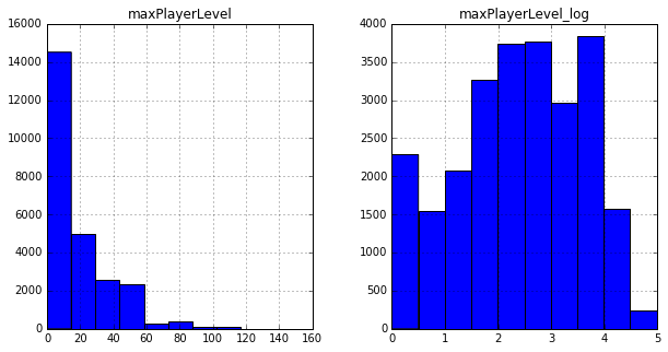
For example, it was noticed that the distribution of many signs resemble logarithmic ones, so I added their logarithms (or rather log (x + 1)) to the base columns.
Then I generated various functions from all possible combinations of the two columns and checked how they affect the result. Within the framework of this task, it seemed to me pointless to invent some “interpretable” signs, because it would be much faster to simply sort them out, since the amount of data allows. A good result, for example, was given by the differences of various signs, which made it possible to get 0.3819 on the same xgboost.
About optimization of parameters and selection of columns can be read in my previous article .
When checking the solutions at the very beginning of the championship, it turned out that the change in the evaluation on the leaderboard is rather bad at the change in the local assessment. When generating new columns, the logloss on the local cross-validation decreased steadily, while on the leaderboard it grew, and no changes in the parameters of the local partitioning of the sample helped to verify. Watching the general chat of the competition, it was possible to notice that a lot of participants encountered this problem, regardless of the means and variances of local estimates. This was another sign in favor of creating an ensemble of models.
On the same set of columns (at this point I got 70 of them), I created two more ensembles of gradient trees, but from other libraries, sklearn and lightgbm . The training took place as follows - at first I tuned each model separately for the best result, then I took the average, saved the results of all models and set up each in turn, but not for my own best result, but for the best result in an ensemble of three models. This gave about 0.3817 on the leaderboard.
Despite the fact that even different implementations of the same algorithms, when averaged in an ensemble, give the best result, it is much more efficient to combine different algorithms together.
So a logistic regression was added to the general ensemble. The model was built in the same way as the past - we generate all possible signs, recursively select and leave the best ones. Here I was disappointed. The local regression performed better than xgboost! The score on the leaderboard was much worse: 0.383. I struggled with this for a long time, threw out the signs in which the distribution on the training and test samples were different, tried various methods of normalization, tried to break the signs into intervals - nothing helped. But even with this result, adding regression to the ensemble turned out to be useful - the result is approximately 0.3816
Since linear regression has shown a good result, it is worth trying neural networks. I spent enough time on them, since the application of standard hyperoptimization algorithms to the structure of a neuron network gives a very weak result. As a result, a good configuration was found which gave about as much on the leaderboard as the regression. The keras library was used for implementation, I will not give the structure here, you can find it in the final file, I will give just a small sample of code that helped me a lot. At the cross-training it was clear that the result of the model strongly depends on the number of epochs of training. You can reduce the learning rate - but it worsened the result, I did not succeed in adjusting the decay - the result was also worsened. Then I just decided to change the learning rate once in the middle of training.
The result after adding to the ensemble - the result is approximately 0.3815.
All the above models were built on approximately the same columns - generated on the basis of basic features and their logarithms. I also tried to generate attributes based on the base columns and their square roots. This also helped - two more ensembles of gradient trees were added. Such a set became final: regression, neural network and five ensembles of gradient trees. The result is approximately 0.3813
An important addition to the ensemble was a slight change in the overall result of the model before shipping. It was found that in the training sample there are large groups of lines with exactly the same signs. And since logloss urges us to optimize the probability, it would be logical to replace the model results on these groups with the average calculated on the training sample. This was done for groups of more than 50 elements. The result is approximately 0.3809
Stacking With such a large number of models, it seems that you can think of a better function for averaging them than a simple arithmetic average. You can, for example, put their results in another model. I refused this idea because the local results did not coincide strongly with the leaderboard, and even the simplest type of stacking did not work - the weighted average.
Manual change of results. On the training sample met subgroups whose results were strictly 1 or strictly 0, for example, all players played 14 days. Then of course it was worth remembering how badly the logloss punishes for such values; in the case of use, more than one hundred places could be lost.
Until the last moment, among the models there was also a random forest, but in the end, based on the public score, I excluded it, although, as it turned out, the privat score showed the model with the best result.
As a result, I really want to thank the organizers! Here you can see the source code of the solution.
I introduce myself, my name is Karachun Mikhail, I am also the winner of the previous contest mail.ru. My past decision is described here and sometimes I will refer to it.
Conditions
The participants of the competition were asked to predict the probability that the player who played the online game would leave it on the basis of a sample of data. The sample contained some data on the activity of the players for two weeks, logloss was selected as a metric, a detailed description of the problem on the competition website .
Introduction
Each machine learning competition has its own specifics, which depends on the data sample offered by the participants. This can be a huge table of raw logs that need to be cleaned and converted into signs. This can be a whole database with different tables from which you also need to generate features. In our case, there was very little data (25k rows and 12 columns), they were free of gaps and errors. Based on this, the following assumptions were made:
')
- It is more efficient to generate and sort hypotheses than to invent them, since the amount of data is very small.
- Most likely in the sample there is no one very cool hidden dependency that will eventually solve everything (killer feature).
- Most likely the struggle will be for the n-th decimal place and the top 10 will be very tight.
That is, it should have been a competition in which it is difficult to find a good dependence in the data and the best solution would consist more of an ensemble of models than of a single one. So it happened.
A small lyrical digression. Most winning decisions of machine learning contests are not suitable for real-world systems. To take at least the well-known case with Netflix, they paid $ 1 million for a solution that they could not implement . Therefore, the final models in such contests remind me of one novel. The second part of its name “Modern Prometheus” is the one that brought people fire and knowledge. The first part, of course, "Frankenstein".
Basic solution
As a base solution, I used xgboost which, after optimizing parameters through hyperopt, immediately gave the result on a 0.3825 leaderboard. Next, I moved to feature engineering.
For example, it was noticed that the distribution of many signs resemble logarithmic ones, so I added their logarithms (or rather log (x + 1)) to the base columns.
Then I generated various functions from all possible combinations of the two columns and checked how they affect the result. Within the framework of this task, it seemed to me pointless to invent some “interpretable” signs, because it would be much faster to simply sort them out, since the amount of data allows. A good result, for example, was given by the differences of various signs, which made it possible to get 0.3819 on the same xgboost.
About optimization of parameters and selection of columns can be read in my previous article .
First trouble
When checking the solutions at the very beginning of the championship, it turned out that the change in the evaluation on the leaderboard is rather bad at the change in the local assessment. When generating new columns, the logloss on the local cross-validation decreased steadily, while on the leaderboard it grew, and no changes in the parameters of the local partitioning of the sample helped to verify. Watching the general chat of the competition, it was possible to notice that a lot of participants encountered this problem, regardless of the means and variances of local estimates. This was another sign in favor of creating an ensemble of models.
More trees ...
On the same set of columns (at this point I got 70 of them), I created two more ensembles of gradient trees, but from other libraries, sklearn and lightgbm . The training took place as follows - at first I tuned each model separately for the best result, then I took the average, saved the results of all models and set up each in turn, but not for my own best result, but for the best result in an ensemble of three models. This gave about 0.3817 on the leaderboard.
Regression
Despite the fact that even different implementations of the same algorithms, when averaged in an ensemble, give the best result, it is much more efficient to combine different algorithms together.
So a logistic regression was added to the general ensemble. The model was built in the same way as the past - we generate all possible signs, recursively select and leave the best ones. Here I was disappointed. The local regression performed better than xgboost! The score on the leaderboard was much worse: 0.383. I struggled with this for a long time, threw out the signs in which the distribution on the training and test samples were different, tried various methods of normalization, tried to break the signs into intervals - nothing helped. But even with this result, adding regression to the ensemble turned out to be useful - the result is approximately 0.3816
Neural networks
Since linear regression has shown a good result, it is worth trying neural networks. I spent enough time on them, since the application of standard hyperoptimization algorithms to the structure of a neuron network gives a very weak result. As a result, a good configuration was found which gave about as much on the leaderboard as the regression. The keras library was used for implementation, I will not give the structure here, you can find it in the final file, I will give just a small sample of code that helped me a lot. At the cross-training it was clear that the result of the model strongly depends on the number of epochs of training. You can reduce the learning rate - but it worsened the result, I did not succeed in adjusting the decay - the result was also worsened. Then I just decided to change the learning rate once in the middle of training.
from keras.callbacks import Callback as keras_clb class LearningRateClb(keras_clb): def on_epoch_end(self, epoch, logs={}): if epoch ==300: self.model.optimizer.lr.set_value(0.01) The result after adding to the ensemble - the result is approximately 0.3815.
More models for God models
All the above models were built on approximately the same columns - generated on the basis of basic features and their logarithms. I also tried to generate attributes based on the base columns and their square roots. This also helped - two more ensembles of gradient trees were added. Such a set became final: regression, neural network and five ensembles of gradient trees. The result is approximately 0.3813
Sample analysis
An important addition to the ensemble was a slight change in the overall result of the model before shipping. It was found that in the training sample there are large groups of lines with exactly the same signs. And since logloss urges us to optimize the probability, it would be logical to replace the model results on these groups with the average calculated on the training sample. This was done for groups of more than 50 elements. The result is approximately 0.3809
Ideas that I refused
Stacking With such a large number of models, it seems that you can think of a better function for averaging them than a simple arithmetic average. You can, for example, put their results in another model. I refused this idea because the local results did not coincide strongly with the leaderboard, and even the simplest type of stacking did not work - the weighted average.
Manual change of results. On the training sample met subgroups whose results were strictly 1 or strictly 0, for example, all players played 14 days. Then of course it was worth remembering how badly the logloss punishes for such values; in the case of use, more than one hundred places could be lost.
Until the last moment, among the models there was also a random forest, but in the end, based on the public score, I excluded it, although, as it turned out, the privat score showed the model with the best result.
As a result, I really want to thank the organizers! Here you can see the source code of the solution.
Source: https://habr.com/ru/post/324916/
All Articles