Tensorflow deep learning library

Hello, Habr! The series of articles on learning tools for neural networks continues with an overview of the popular Tensorflow framework.

Tensorflow (hereinafter referred to as TF) is a rather young framework for deep machine learning developed by Google Brain. For a long time, the framework was developed in a closed mode under the name DistBelief, but after a global refactoring on November 9, 2015 it was released in open source. In a year with a little TF, it grew to version 1.0, gained integration with keras, became much faster and received support for mobile platforms. Recently, the framework has also been developing towards classical methods, and in some parts of the interface it is already somewhat reminiscent of scikit-learn. Prior to the current version, the interface changed actively and often, but the developers promised to freeze changes to the API. We will consider only the Python API, although this is not the only option - there are also interfaces for C ++ and mobile platforms.

Installation

TF is installed as standard via python pip. There is a nuance: there are separate installation algorithms for operation on the CPU and on the video cards.

In the case of the CPU, everything is simple: you need to put a pip package called tensorflow.

In the second case, you need:

1. check compatibility with video card. The CUDA Compute Capability parameter should be greater than 3.0, you can find it for your video card here.
2. Install CUDA Toolkit Eighth Version
3. Install cuDNN version 5.1
4. Install tensorflow-gpu package from pip

However, the documentation claims that earlier versions of CUDA Toolkit and cuDNN are supported, but recommends installing the versions mentioned above.

Developers recommend installing TF in a separate environment with virtualenv to avoid possible problems with versioning and dependencies.

Another installation option is Docker. By default, only the CPU version will work from the container, but if you use the special nvidia docker , then you can use the GPU.

I did not try it myself, but they say that TF even works with Windows. Installation is carried out through the same pip and, they say, works without problems.

I skip the build process from source, but this option may make sense. The fact is that the package from the repository is assembled without the support of SSE and other buns. In the latest versions, TF checks for the presence of such buns and reports that it will run faster from the sources.

The installation process is described in detail here .

Documentation

There is a lot of documentation and examples.

• Official site
• Official Tutorials
• Awesome-list - a selection of all the best on the topic
• Excellent collection of different models on TF

The best way to focus on official documentation is that due to the rapid development and frequent changes of api, there are a lot of tutorials and scripts on the Internet that target the old versions (well, like the old ... half a year ago) with the old API, they will not work with the latest versions of the framework .

Basic TF Elements

With the help of "Hello, world" we will make sure that everything was established correctly:

import tensorflow as tf #  TF hello = tf.constant('Hello, TensorFlow!') #    TF sess = tf.InteractiveSession() #   print(sess.run(hello)) # ""  >>> b'Hello, TensorFlow!' 

The first line we connect TF. The rule has already been established to introduce a corresponding abbreviation for the framework. This same piece of code is found in the documentation and allows you to make sure that everything was installed correctly.

Computation graph

Work with TF is built around building and executing a graph of calculations. The computation graph is a construct that describes how calculations will be performed. In classical imperative programming, we write code that is executed line by line. In TF, the usual imperative approach to programming is needed only for some auxiliary purposes. The basis of TF is the creation of a structure defining the order of calculations. Programs are naturally structured into two parts - the compilation of a graph of calculations and the execution of calculations in the structures created.

The computation graph in TF does not differ in meaning from that in Theano. In the previous article of the cycle an excellent description of this entity is given.

A TF graph consists of placeholders, variables, and operations. From these elements it is possible to collect a graph in which the tensors will be calculated. Tensors are multidimensional arrays; they serve as a “fuel” for a graph. A tensor can be either a single number, a feature vector from the problem being solved or an image, or a whole batch of object descriptions or an array of images. Instead of a single object, we can transfer to the graph an array of objects and an array of answers will be computed for it. TF work with tensors is similar to how it processes numpy arrays, in functions of which you can specify the axis of the array relative to which the calculation will be performed.

Sessions

Computing graphs are performed in sessions. The session object ( tf.Session ) hides in itself the execution context of the graph - the necessary resources, auxiliary classes, address spaces.
There are two types of sessions - regular, which are implemented in tf.Session and interactive ( tf.InteractiveSession ). The difference between them is that an interactive session is more suitable for execution in the console and immediately defines itself as a default session. The main effect is that the session object does not need to be passed to the calculation function as a parameter. In the examples below, I will assume that the interactive session is currently running, which we announced in the first example, and when I need to refer to the session, I will refer to the sess object.

Further, in the post, standard TF images with graph images will appear, generated by a built-in utility called Tensorboard. The designations there are:

Variable	Operation	Auxiliary result
The graph node usually contains data.	Does something with variables. This also includes placeholders who make the substitution of values ​​in the graph.	Any caching and side calculations of the type of gradients, usually refer to a separate part of the graph.

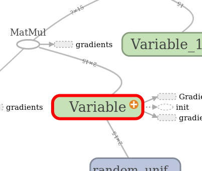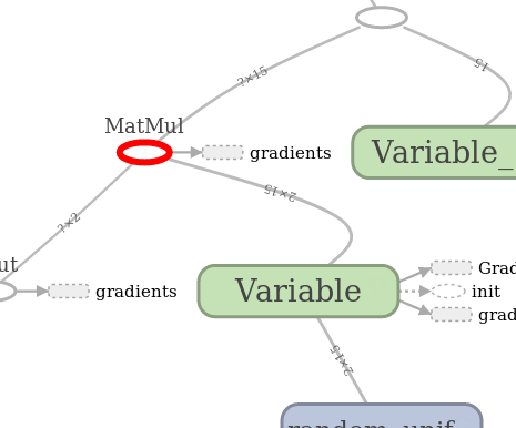Tensors, operations and variables

For example, create a tensor filled with zeros.

 zeros_tensor = tf.zeros([3, 3]) 

In general, the API in TF will largely resemble numpy and tf.zeros() — far from the only function that has a direct analogue in numpy. To see the value of the tensor, it must be executed. In more detail about performance of the graph slightly below, so far we will manage that we will display the value of the tensor and the tensor itself.

 print(zeros_tensor.eval()) print(zeros_tensor) >>> [[ 0. 0. 0.] [ 0. 0. 0.] [ 0. 0. 0.]] >>> Tensor("zeros_1:0", shape=(3, 3), dtype=float32) 

The difference between the lines is that the tensor is calculated in the first line, and in the second line we just print the object representation.

The tensor description shows us several important things:

1. The tensors have names. At our zeros it: 0
2. There is a notion of the form of a tensor, it looks like the dimension of an array of numpy.
3. The tensors are typed and the types for them are set from the library.

Above tensors, you can perform a variety of operations:

 a = tf.truncated_normal([2, 2]) b = tf.fill([2, 2], 0.5) print(sess.run(a + b)) print(sess.run(a - b)) print(sess.run(a * b)) print(sess.run(tf.matmul(a, b))) >>> [[-1.12130964 -1.02217746] [ 0.85684788 0.5425666 ]] >>> [[ 0.35249496 0.96118248] [-1.55395389 -1.18111515]] >>> [[-0.06559008 -0.11100233] [ 0.51474923 -0.27813852]] >>> [[-0.16202734 -0.16202734] [-0.8864761 -0.8864761 ]] 

In the example above, we use the sess.run construct — this is the method for executing graph operations in a session. In the first line, I created a tensor from a truncated normal distribution. It uses the standard generation of the normal distribution, but it excludes everything that falls outside the limits of two standard deviations. In addition to this generator, there is a uniform, simple normal, gamma, and several other distributions. A very characteristic thing for TF - most of the popular options for performing an operation have already been implemented and, perhaps, before inventing a bicycle, you should look at the documentation. The second tensor is a multidimensional 2x2 array filled with a value of 0.5 and this is something similar to numpy and its functions of creating multidimensional arrays.

Now let's create a variable based on the tensor:

 v = tf.Variable(zeros_tensor) 

The variable participates in the calculations as a node of the computational graph, saves the state, and it needs some initialization. So, if in the next example we do without the first line, then TF will throw an exception.

 sess.run(v.initializer) v.eval() >>> array([[ 0., 0., 0.], [ 0., 0., 0.], [ 0., 0., 0.]], dtype=float32) 

Operations on variables create a computational graph, which can then be performed. There are also placeholders - objects that parameterize the graph and mark places for the substitution of external values. As written in the official documentation, a placeholder is a promise to substitute value later. Create a placeholder and assign it a data type and size:

 x = tf.placeholder(tf.float32, shape=(4, 4)) 

Another such use example. Here, two placeholders serve as input nodes for the adder:

 a = tf.placeholder("float") b = tf.placeholder("float") y = tf.multiply(a, b) print(sess.run(y, feed_dict={a:100, b:500})) >>> 50000.0 

Simple calculations.

As an example, create and calculate several expressions.

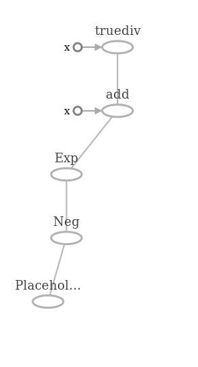
 x = tf.placeholder(tf.float32) f = 1 + 2 * x + tf.pow(x, 2) sess.run(f, feed_dict={x: 10}) >>> 121.0 

And the calculation graph:

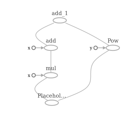
x and y points to the operations in this scheme are additional parameters that could be replaced by graph edges, but we substituted scalar values ​​1 and 2 into f and this is just a designation in the graph for numbers. In this example, we create a placeholder and, based on it, an expression graph $$$1 + 2x + x ^ 2$, and then we perform graph calculations in the context of the current session. I did not specify the form in the placeholder parameters and this means that tensors of any sizes can be fed to the input. The only thing you need to specify is the type of tensor. The parameters for the calculation inside the session are transmitted through the feed_dict dictionary with all that is necessary for the calculations.

Let's try to collect something more practically meaningful.
For example, sigmoid: $$$\ sigma (x) = \ frac {1} {1 + e ^ {- x}}$

 x = tf.placeholder(dtype=tf.float32) sigma = 1 / (1 + tf.exp(-x)) sigma.eval(feed_dict={x: np.linspace(-5, 5) }) 

And such a graph for her.

In the fragment with the launch of the calculation function, there is one thing that distinguishes this example from the previous ones. The fact is that in the placeholder, instead of a single scalar value, we pass a whole array. TF processes all the values ​​of the array together, within the same tensor (remember that the array == tensor). In exactly the same way, we can transfer objects to the graph in whole batchy and deliver images to the neural network as a whole.

In general, working with tensors resembles working with arrays in numpy. However, there are some differences. When we want to lower the dimension, somehow combining the values ​​in the tensor for a certain dimension, we use those functions that begin with reduce_ .
If you compare the Theano API - in TF there is no division by vectors and matrices, but instead you have to follow the dimensions of the tensors in the graph and there is a mechanism for deriving the form of the tensor, which allows you to get dimensions even before runtime.

Machine learning

Let us first analyze the classical linear regression mentioned here more than once, with a detailed description of which can be found here , but we will use the gradient descent method for teaching.

Where do without this picture

I'll start with linear regression, and then add polynomial features.
The data will be synthetic - sine with normal noise:

 x = np.linspace(0, 10, 1000) y = np.sin(x) + np.random.normal(size=len(x)) 

They will look something like this:

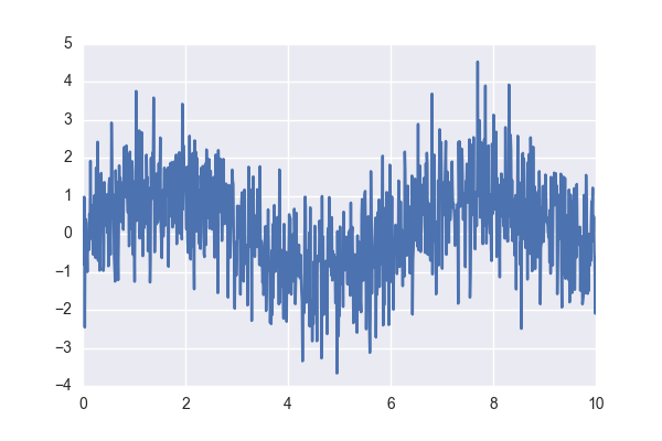
I will still break the sample into a training and reference in the proportion of 70/30, but I will leave this and some other routine points in the full source, the link to which will be slightly lower.

First, we construct a simple linear regression.

 x_ = tf.placeholder(name="input", shape=[None, 1], dtype = tf.float32) y_ = tf.placeholder(name= "output", shape=[None, 1], dtype = tf.float32) model_output = tf.Variable(tf.random_normal([1]), name='bias') + tf.Variable(tf.random_normal([1]), name='k') * x_ 

Here I create two placeholders for the sign and the answer and the formula of the form $$$kx + b$.
Nuance - in the placeholder the shape parameter (shape) contains None. The dimension of the placeholder means that the pleisoder consumes two-dimensional tensors, but on one of the axes the size of the tensor is not defined and can be any. This is done so that the user can transfer the values ​​to the graph at once in whole batch. Such specific dimensions are called dynamic, TF calculates the actual dimension of related elements during the execution of the graph.

The placeholder for the sign is used in the formula, but for the answer, I place the placeholder for the loss function $$$\ frac {1} {n} \ sum ^ {n} _ {i = 1} (y_i - \ hat {y} _i) ^ 2$:

 loss = tf.reduce_mean(tf.pow(y_ - model_output, 2)) #   

In TF implemented a dozen methods of optimization. We will use the classic gradient descent, indicating the speed of learning in the parameters.

The minimize method will create an operation for us, the calculation of which will minimize the loss function.

 gd = tf.train.GradientDescentOptimizer(0.001) # train_step = gd.minimize(loss) 

Initialization of variables - it is necessary for further calculations:

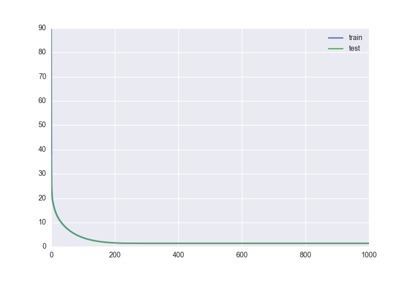
 sess.run(tf.global_variables_initializer()) 

Everything can finally be taught. I will launch 100 epochs of training on the training part of the sample, after each training I will arrange control on the delayed part.

 n_epochs = 100 train_errors = [] test_errors = [] for i in tqdm.tqdm(range(n_epochs)): # 100 _, train_err = sess.run([train_step, loss ], feed_dict={x_:X_Train.reshape((len(X_Train), 1)) , y_: Y_Train.reshape((len(Y_Train), 1))}) train_errors.append(train_err) test_errors.append(sess.run(loss, feed_dict={x_:X_Test.reshape((len(X_Test), 1)) , y_: Y_Test.reshape((len(Y_Test), 1))})) 

The first session execution of the train_step and loss operations at the same time does both the training and the error estimate on the training set, i.e. proper assessment of how well we memorized the sample. The second session execution is counting losses on the test sample. In the feed_dict parameter feed_dict I pass values ​​to the graph for placeholders and reshape to ensure that the data arrays are the same in size. Where the value of None in the placeholder, any number can be passed. Tensors with such uncertain sizes are called dynamic, and here I use them to transfer to the graph batchy with examples for training.

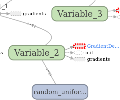
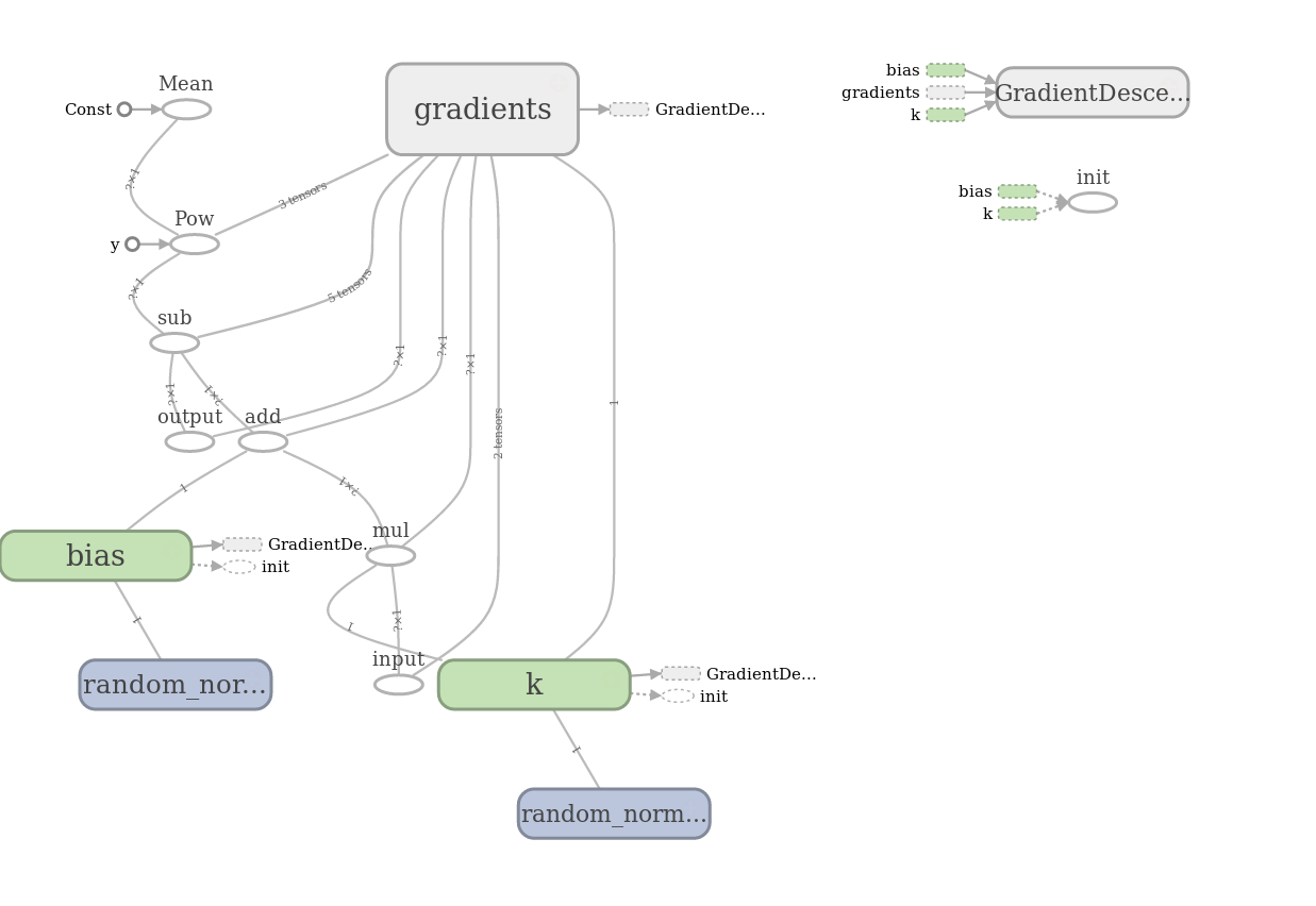
It turns out this is the dynamics of learning:

In this column there are auxiliary variables with gradients and initialization operations, they are placed in a separate block.

And here are the model calculation results:

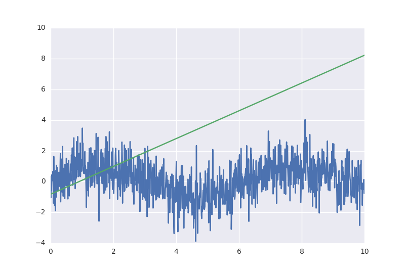
I calculated the values ​​for the graph in this way:

 sess.run(model_output, feed_dict={x_:x.reshape((len(x), 1))}) 

Here, in the graph, I pass the value only to the x_ placeholder - the rest is simply not necessary to evaluate the model_output expression.

Full listing of the program is here . The result was predictable for such a simple linear model.

Polynomial regression

Let us try to diversify the regression with polynomial signs, regularization, and changes in the model learning speed.

In the generation of a dataset, we add a certain number of degrees and normalize the features using PolynomialFeatures and StandardScaler from the scikit-learn library. The first object will create as many polynomial signs as we want, and the second normalizes them.

For the transition to polynomial regression, we replace only a few lines in the graph of calculations:

 order = 26 #   x_ = tf.placeholder(name="input", shape=[None, order], dtype=tf.float32) y_ = tf.placeholder(name= "output", shape=[None, 1], dtype=tf.float32) w = tf.Variable(tf.random_normal([order, 1]), name='weights') model_output = tf.matmul(x_, w) 

In fact, we now consider $$$model_ {output} = \ sum ^ {order} _ {i = 1} x ^ i \ dot w_i$. Obviously, there is a danger of retraining the model on level ground, so we will add regularization penalties on weights. Penalties are added to the loss function (loss in the examples) as additional terms and we get almost ElasticNet from sklearn.

$$

$$loss = \ frac {1} {n} \ sum ^ {n} _ {i = 1} (y_i - \ hat {y} _i) ^ 2 + \ alpha \ sum {w} ^ 2 + \ beta \ sum | w |$$

 loss = tf.reduce_mean(tf.square(y_ - model_output)) + 0.85* tf.nn.l2_loss(w) + 0.15* tf.reduce_mean(tf.abs(w)) 

For the most popular L2 regression, there is a separate function l2_loss , but the selection of features using L1 will have to be implemented manually, but we will have this average over all absolute weights.

For the sake of example, I will add another significant change that will affect the pace of learning. Quite often, when training heavy neural networks, this is simply a necessary measure in order to avoid learning problems and get an acceptable result. A very simple idea - as you learn to gradually lower the parameter of a step, avoiding big trouble.

Instead of a constant rate, we will use the exponential decay, which I took straight from the documentation:

 learning_rate = tf.train.exponential_decay(starter_learning_rate, global_step, 100000, 0.96, staircase=True) 

Inside the function, there is a formula:

$$

$$learning \ _rate_ {decayed} = learning \ _rate * decay \ _rate ^ {\ frac {global \ _step} {decay \ _steps}}$$

In our example, decay_rate is set to 100000, decay_rate is 0.96.

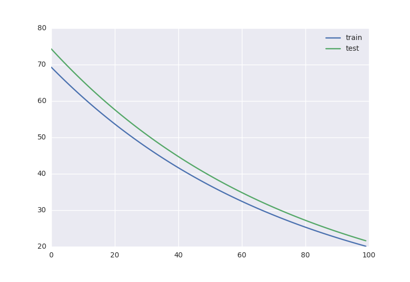
We get the following rates of error reduction in training and control:

In addition to the exponential decay, there are other functions that allow you to reduce the speed of learning, and of course nothing prevents you from creating another function to fit your needs.

The model itself after training and various selections of parameters will look something like this:

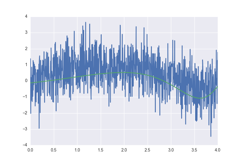
To obtain this result, I changed the coefficients at regularization and learning speed. Enumerating the values ​​of constants in the loss formula is a great way to see with your own eyes the effect of the regularizers, I highly recommend playing with the settings in the full polynomial regression source, it is available here .

Saving and loading graphs

We got a model and it would be nice to keep it. In TF, everything is quite simple - the API has a special serializer object that does two things:

1. Saves the current graph, its state and variable values ​​to a file;
2. Reads all the same from a file.

All you need to do is create this object:

 saver = tf.train.Saver() 

The state of the current session is saved using the save method:

 saver.save(sess, "checkpoint_dir/model.ckpt") 

It is already somehow accepted that the saved states of the model are called checkpoints, hence the name of the folders and file extensions. Recovery is performed using the restore method:

 ckpt = tf.train.get_checkpoint_state(ckpt_dir) if ckpt and ckpt.model_checkpoint_path: print(ckpt.model_checkpoint_path) saver.restore(session, ckpt.model_checkpoint_path) 

First, using a special function, we get the state of the checkpoint (if all of a sudden there is no saved model in the target directory, the function will return None ). By default, the function looks for a checkpoint file, but this behavior can be changed using the parameter. After this, restore restores the state of the graph.

Tensorboard

The extremely useful system in the TF is a web-dashboard, which allows you to collect statistics from dumps and logs and observe what happens during the calculations. It is extremely convenient that the dashboard runs on a web server and, for example, you can run tensorboard on a remote machine in the cloud and watch what is happening in your browser window.

Tensorboard can:

1. Draw a graph of calculations.
   The graph of computations is worth looking at least for a self-test, in order to make sure that what has been collected and considered is exactly what was planned, and no mistakes were made during coding.
2. Show variable statistics.
   You can collect any statistics at all.
3. There is a tool for analyzing multidimensional data (for example, embeddingings).
   To do this, PCA and t-SNE are built into the dashboards, with which you can try to view the data in 2 and 3 dimensions.
4. Histograms
   You can build a histogram of the distribution of the outputs of the network layers and the behavior of variables.

The reverse side of the medal is that in order for the statistics to fall into the dashboards, it must be saved to the logs (in the protobuf format) using a special API. API is not very complex, grouped in tf.summary . To collect statistics, you will need to separately register the variables of interest using special functions and then separately save everything to the log.

Even when using Tensorboard, it is also important not to forget about the name parameter of variables. The name that will be assigned to the variable will then be used to draw the graph, select the user interface of the dashboard, in general, everywhere. For small graphs, this is not critical, but as the complexity of the task grows, problems may arise with understanding what is happening.

There are several types of functions that save variable data in various ways:

 tf.summary.histogram("layer_output", w_h) 

This function will allow you to collect a histogram for the layer exit and approximately estimate the dynamics of changes during training. The tf.summary.scalar("accuracy", learning_rate) function will store a number. You can still save audio and images.

To save the logs you need a little more: you first need to create a FileWriter to write the file.

 writer = tf.summary.FileWriter("./logs/nn_logs", sess.graph) # for 1.0 merged = tf.summary.merge_all() 

And combine all the statistics in one object.

Now we need to transfer this merged object to the session and then use the FileWriter method FileWriter add new data received from the session.

 summary, op_result = sess.run([merged, op], feed_dict={X: X_train, Y: y_train, p_keep_input: 1.0, p_keep_hidden: 1.0}) writer.add_summary(summary, i) 

However, for simple saving of the graph such code is enough:

 merged = tf.summary.merge_all(key='summaries') if not os.path.exists('tensorboard_logs/'): os.makedirs('tensorboard_logs/') my_writer = tf.summary.FileWriter('tensorboard_logs/', sess.graph) 

And a nuance: the default Tensorboard is locally available at 127.0. 1 .1: 6006. I hope I saved the readers a few seconds of time and neurons with this remark.

Multilayer perceptron

Let us analyze the canonical example of memorizing the function xor, which the linear model cannot assimilate due to the impossibility of a linear division of the space of attributes.

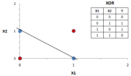
Multilayer networks assimilate the function because they make an implicit conversion of the space of attributes into separable or, depending on the implementation, make a nonlinear partition of this space. We are implementing the first option - we will create a two-layer perceptron with non-linear activation of the layers. The first layer will do the nonlinear transformation, and the second layer is almost linear regression, which works on the transformed feature space.

As an element of nonlinearity, we will use the relu function.

Define the network structure:

 x_ = tf.placeholder(name="input", shape=[None, 2], dtype=tf.float32) y_ = tf.placeholder(name= "output", shape=[None, 1], dtype=tf.float32) hidden_neurons = 15 w1 = tf.Variable(tf.random_uniform(shape=[2, hidden_neurons ])) b1 = tf.Variable(tf.constant(value=0.0, shape=[hidden_neurons ], dtype=tf.float32)) layer1 = tf.nn.relu(tf.add(tf.matmul(x_, w1), b1)) w2 = tf.Variable(tf.random_uniform(shape=[hidden_neurons ,1])) b2 = tf.Variable(tf.constant(value=0.0, shape=[1], dtype=tf.float32)) nn_output = tf.nn.relu(tf.add(tf.matmul(layer1, w2), b2)) 

keras , TF, Theano . , , dropout- , , ( , , ).

, :

 def fully_connected(input_layer, weights, biases): layer = tf.add(tf.matmul(input_layer, weights), biases) return(tf.nn.relu(layer)) 

: - ( — ) , tensorboard - .

:

 gd = tf.train.GradientDescentOptimizer(0.001) loss = tf.reduce_mean(tf.square(nn_output - y_)) train_step = gd.minimize(loss) 

:

 x = np.array([[0, 0], [1, 0], [0, 1], [1, 1]]) y = np.array([[0], [1], [1], [0]]) for _ in range(20000): sess.run(train_step, feed_dict={x_:x, y_:y}) 

:

: , . , — . , , .

, . :

 sess.run(nn_output, feed_dict={x_:x}) 

. 5 .

, TF .

, . Tesla, - . TF . «/cpu:0», «/gpu:0» .. — , «» :

 with tf.device('/cpu:0'): a = ... 

.

, . :

 cfg = tf.ConfigProto() sess = tf.Session(config=cfg) 

log_device_placement , , .

, GPU. :

 gpu_opts = tf.GPUOptions(per_process_gpu_memory_fraction = 0.25) sess = tf.Session(config=tf.ConfigProto(gpu_options = gpu_opts)) 

GPU, , , CPU, allow_soft_placement , TF . API . , — , .

Conclusion

TF - , , . , , -. , «» . TF Kaggle!

sovcharenko , Ferres bauchgefuehl .

UPD:
Jupyter- .