On linear regression: Bayesian approach to the ruble exchange rate

It is no secret that the ruble exchange rate directly depends on the cost of oil (and on something else). This fact allows you to build quite interesting models. In my article on linear regression, I touched upon some questions devoted to the diagnosis of the model, but the question behind the scenes was: is there a more efficient, but not too complicated, alternative to linear regression? The traditionally used least squares method is simple and straightforward, but there are other approaches. (not so clear) .

MNC data and diagnostics

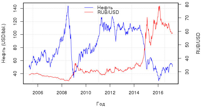
In this article, we will compare several models that are linear in nature, using the dependence of the ruble exchange rate on the cost of oil as a visual aid. Remember this wonderful post ? After two years, it is time to update the graphics. We’ll download the latest data from Quandl : behind the "EIA / PET_RBRTE_D" code lies the spot price for Brent crude in $, and for "BOE / XUDLBK69" - the cost of 1 dollar in Russian rubles.

library(Quandl) library(zoo) library(dplyr) oil.ts <-Quandl("EIA/PET_RBRTE_D", trim_start="2005-04-03", trim_end="2017-03-10", type="zoo", collapse="weekly") usd.ts <-Quandl("BOE/XUDLBK69", trim_start="2005-04-03", trim_end="2017-03-10", type="zoo", collapse="weekly") 

The time interval is from April 2005 to March 2017. And what is the dynamics observed during this period, if we express the value of the ruble in dollars:

Judging by the schedule, the relationship between the curves of the value of the ruble and oil was traced constantly, but after 2012 it became especially close. In principle, there is not much point in building one regression of the OLS for all these years, because due to sharp price fluctuations, the regression residuals will have a multimodal distribution, and you will get a model that describes everything badly. Therefore, we consider the period from March 2015 to December 2016 - this will be a training set; data for 2017 is used for testing.

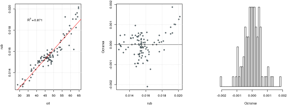
The nature of the relationship since 2015 has not changed, and the linear regression rub _i = a + b · oil _i , constructed using OLS is statistically significant:

 tr.s <- "2015-03-01"; tr.e <- "2016-12-31" train <- data.frame(oil=as.vector(window(oil.ts, start=tr.s, end=tr.e)), rub=as.vector(window(rub.ts, start=tr.s, end=tr.e)), date=index(window(oil.ts, start=tr.s, end=tr.e))) %>% mutate(month=factor(format(date, "%m")), date=NULL) te.s <- "2017-01-01"; te.e <- "2017-03-15" test <- data.frame(oil=as.vector(window(oil.ts, start=te.s, end=te.e)), rub=as.vector(window(rub.ts, start=te.s, end=te.e)), date=index(window(oil.ts, start=te.s, end=te.e))) %>% mutate(month=factor(format(date, "%m")), date=NULL) fit1 <- lm(rub ~ oil, data=train) summary(fit1) ## ## Call: ## lm(formula = rub ~ oil, data = train) ## ## Residuals: ## Min 1Q Median 3Q Max ## -2.096e-03 -3.265e-04 4.510e-06 3.491e-04 1.871e-03 ## ## Coefficients: ## Estimate Std. Error t value Pr(>|t|) ## (Intercept) 7.284e-03 3.396e-04 21.45 <2e-16 *** ## oil 1.777e-04 7.009e-06 25.35 <2e-16 *** ## --- ## Signif. codes: 0 '***' 0.001 '**' 0.01 '*' 0.05 '.' 0.1 ' ' 1 ## ## Residual standard error: 0.0005883 on 94 degrees of freedom ## Multiple R-squared: 0.8724, Adjusted R-squared: 0.871 ## F-statistic: 642.7 on 1 and 94 DF, p-value: < 2.2e-16 

If you remove the free term, then R ² will be almost equal to one. There is an explanation . No matter how tempting it may be, one cannot just zero out a free member (unless the process being studied ensures that the regression line passes through the origin): if you are interested, you can read here . You should not dwell on R ² - this criterion is quite formal . As for the remnants of the model, they are generally well distributed, but it seems to be bimodal:

 library(lmtest) dwtest(fit1) ## ## Durbin-Watson test ## ## data: fit1 ## DW = 0.49421, p-value < 2.2e-16 ## alternative hypothesis: true autocorrelation is greater than 0 resettest(fit1) ## ## RESET test ## ## data: fit1 ## RESET = 13.999, df1 = 2, df2 = 92, p-value = 4.924e-06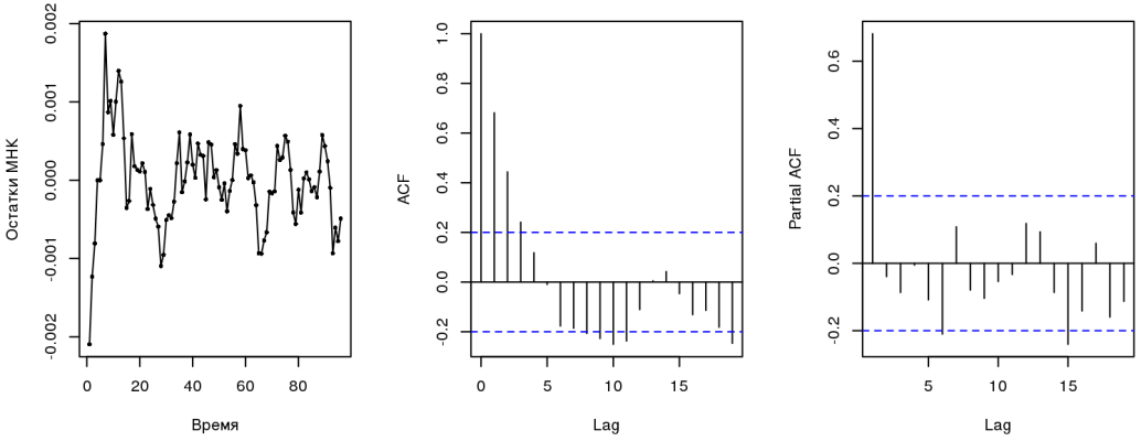 

The Darbin-Watson test indicates the presence (who would have thought) of autocorrelation ; residual correlograms indicate an AR (1) process (we’ll talk about this later). RESET test indicates the missing variables, which is logical, because Many factors influence the course (or MNCs are not the most appropriate model). All this together violates the prerequisites that underlie OLS . The one who is engaged in econometrics will say that it is necessary to use such regression carefully, since all estimates are biased and untenable, it is impossible to build confidence intervals. Of all the properties, only linearity is preserved.

You can also do this trick: it’s possible that the dependency is not linear, but also includes polynomial terms. How to choose a more or less optimal model? You will have to use either cross-validation or information criteria like AIC . For the linear model, I like the latter more, especially since the results of AIC and CV converge asymptotically. The code below performs just what you need: polynomial regressions are constructed with a degree from 1 to 5, and the optimal model is determined based on the minimum of the AIC criterion. The poly () function builds orthogonal polynomials , and they should be used in regression.

 which.min(sapply(1:5, function(i) AIC(lm(rub ~ poly(oil, i), data=train)))) ## [1] 3 

Thus, it turns out that the model can have the following form:

Time series and errors

You can talk about time series infinitely and with varying success . We need to know this. Both the ruble exchange rate and the cost of oil are time series, and this cannot be ignored (hence the problems with errors in the OLS). Some processes can be described using a simple first order autoregressive model . This means that the following value in the time series is well described by the previous one, plus a small error:

where ε _t is white noise .
Build the ARIMA model with an additional regressor:

 library(forecast) fit2 <- auto.arima(train$rub, xreg=train$oil) summary(fit2) ## Series: train$rub ## Regression with ARIMA(1,0,0) errors ## ## Coefficients: ## ar1 intercept train$oil ## 0.9123 0.0108 1e-04 ## se 0.0417 0.0004 0e+00 ## ## sigma^2 estimated as 1.274e-07: log likelihood=626.46 ## AIC=-1244.91 AICc=-1244.47 BIC=-1234.65 ## ## Training set error measures: ## ME RMSE MAE MPE MAPE ## Training set 1.424521e-05 0.000351317 0.0002580076 0.02303551 1.610766 ## MASE ACF1 ## Training set 0.7766594 0.02983604 

From the information about this model, you can find out that during the regression rub _i = a + b · oil _i + u _{i, the} errors u _i have an ARIMA (1, 0, 0) autocorrelation structure, i.e. they are just an autoregression model of the first order AR (1).

Since Now the structure of the errors is approximately known, try the generalized least squares method (GLS) . GLS uses a simple idea as follows. If in solving the system y = Xb + ε by the least squares method, the coefficients of the regressors and the covariance matrix are found from the equations

then when using GLS the corresponding equations will look like this:

Here Σ is the covariance error matrix, which can be estimated by knowing their structure. In theory, such a model gives unbiased , effective , consistent, and asymptotically normal estimates ( Aitken's theorem ).

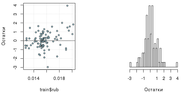
 library(nlme) fit3 <- gls(rub ~ oil, data=train, correlation=corAR1(value=0.7, form=~1|month)) summary(fit3) ## Generalized least squares fit by REML ## Model: rub ~ oil ## Data: train ## AIC BIC logLik ## -1173.847 -1163.674 590.9237 ## ## Correlation Structure: AR(1) ## Formula: ~1 | month ## Parameter estimate(s): ## Phi ## 0.7478772 ## ## Coefficients: ## Value Std.Error t-value p-value ## (Intercept) 0.007860934 0.0004055443 19.38366 0 ## oil 0.000163683 0.0000081087 20.18601 0 ## ## Correlation: ## (Intr) ## oil -0.952 ## ## Standardized residuals: ## Min Q1 Med Q3 Max ## -2.96100735 -0.41075284 0.07903953 0.62870157 3.42607023 ## ## Residual standard error: 0.0006099571 ## Degrees of freedom: 96 total; 94 residual 

You can also check whether we will get any benefit from the inclusion of polynomial members in GLS according to the AIC criterion:

 which.min(sapply(1:5, function(i) { d <- data.frame(poly(train$oil, i), month=train$month, rub=train$rub) AIC(gls(rub ~ . - month, data=d, correlation=corAR1(value=0.7, form=~1|month))) })) ## [1] 1 

Now there is enough regressor in 1 degree. And, by the way, the corrected model errors themselves are more interestingly distributed (although it is impossible not to note the presence of outliers):

Bayes regression and probabilistic choice of variables

At this point, we have three models: OLS, ARIMA (1, 0, 0), GLS with errors AR (1). Now we will consider the problem from the other side and in a different formulation, asking first of all the question of whether we need, for example, polynomial terms:

It is written here that the variable y _{i is} distributed normally and linearly depends on the degrees x _i . In turn, the regression coefficients are not just distributed normally, but can also be "absent" in the equation, which is provided by the indicator variable I _j , which obeys the Bernoulli distribution with the parameter p, i.e. can take only the values ​​0 or 1. The parameter p, in turn, is taken from the beta distribution , and the parameters τ and τ _b - from gamma . So we set a priori distributions . Where do their exact forms come from? This is where the theory is not very intelligible and suggests either to rely on our practical concepts about the nature of the described processes or intuition, or to specify non-informative a priori distributions . Fortunately, the more data is available, the less output depends on a priori distributions. And it becomes clear if you look at the Bayes formula , which is a rule according to which a priori distributions change when certain data is observed:

Here p (θ | y) is the posterior distribution , p (y | θ) is the likelihood , p (θ) is the prior distribution. Then you can write:

And then by inertia:

But it is still desirable that the distributions be more or less meaningful. So, if you look at the histogram y _i (we have a ruble exchange rate), then you can see a curve resembling a normal distribution (or lognormal ...). As for the regression coefficients, then the choice of the Gaussian distribution is justified by the traditional expectation that they are distributed normally.

Of course, no one wants to engage in a fascinating manual output, so we need a library that allows us to describe the model in terms of a priori distributions. In R, these are rjags , and also wrapper functions from R2jags . All of the above will be written in this form:

 library(R2jags) model1 <- "model { for (i in 1:n) { y[i] ~ dnorm(a + inprod(X[i,], b[]), tau) } for (j in 1:p) { ind[j] ~ dbern(pind) bT[j] ~ dnorm(0, taub) b[j] <- ind[j] * bT[j] } a ~ dnorm(0, 1e-04) tau ~ dgamma(1, 1e-03) taub ~ dgamma(1, 1e-03) pind ~ dbeta(2, 9) }" p <- 5 m.jags1 <- jags(data=list(y=train$rub, X=poly(train$oil, p), n=nrow(train), p=p), parameters.to.save=c("a", "b", "ind"), model.file=textConnection(model1), n.chains=1, n.iter=5000) m.jags1 ## Inference for Bugs model at "5", fit using jags, ## 1 chains, each with 5000 iterations (first 2500 discarded), n.thin = 2 ## n.sims = 1250 iterations saved ## mu.vect sd.vect 2.5% 25% 50% 75% 97.5% ## a 0.016 0.000 0.015 0.015 0.016 0.016 0.017 ## b[1] 0.011 0.007 0.000 0.006 0.013 0.017 0.023 ## b[2] 0.000 0.001 0.000 0.000 0.000 0.000 0.003 ## b[3] 0.000 0.001 0.000 0.000 0.000 0.000 0.000 ## b[4] 0.000 0.001 0.000 0.000 0.000 0.000 0.000 ## b[5] 0.000 0.001 0.000 0.000 0.000 0.000 0.000 ## ind[1] 0.764 0.425 0.000 1.000 1.000 1.000 1.000 ## ind[2] 0.046 0.210 0.000 0.000 0.000 0.000 1.000 ## ind[3] 0.034 0.180 0.000 0.000 0.000 0.000 1.000 ## ind[4] 0.031 0.174 0.000 0.000 0.000 0.000 1.000 ## ind[5] 0.045 0.207 0.000 0.000 0.000 0.000 1.000 ## deviance -848.261 15.731 -876.531 -858.633 -848.740 -838.639 -815.570 ## ## DIC info (using the rule, pD = var(deviance)/2) ## pD = 123.7 and DIC = -724.5 ## DIC is an estimate of expected predictive error (lower deviance is better). 

The conclusion shows that the average values ​​of indicator variables I _j with regression coefficients b ₂ , ..., b _{5 are} an order of magnitude less than I ₁ , which means that such a probabilistic model gives us the right to assume that the ruble exchange rate linearly depends on the cost of oil. Next, we write a simple linear model that takes into account the presence of first order autoregression in errors:

 model2 <- "model { a ~ dt(0, 5, 1) b ~ dt(0, 5, 1) phi ~ dunif(-1, 0.999) tau0 ~ dgamma(1, 1e-03) tau[1] <- tau0 y[1] ~ dnorm(a + b * x[1], tau[1]) for (i in 2:n){ tau[i] <- tau0 + phi * tau[i-1] y[i] ~ dnorm(a + b * x[i], tau[i]) } }" set.seed(123) n <- nrow(test) m.jags2 <- jags(data=list(y=c(train$rub, rep(NA, n)), x=c(train$oil, test$oil), n=nrow(train)+n), parameters.to.save=c("a", "b", "phi", "y"), model.file=textConnection(model2), n.chains=1, n.iter=5000) 

This is the posterior distribution of the model parameters: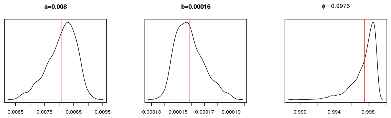

You may notice that they are not much different from the parameters of the GLS model. The regression equation for the average values ​​of the parameters can be written as:

But the 95% probability intervals in the usual form for the predicted values ​​of the dollar in 2017 (the red triangles show the true values):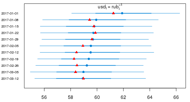

Conclusion

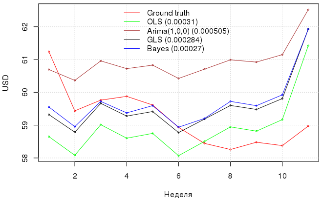
Below is a graph with dollar model predictions and their errors . With such uncomplicated manipulations, we achieved a decrease in MAE from 3.1e-04 for OLS to 2.7e-04 using the Bayesian approach, taking into account the autoregressive process in model errors, and the GLS showed approximately the same result as the Bayesian approach, but with less moral costs. .

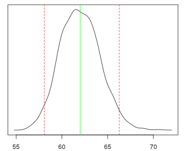
Why bother to turn to such a conclusion at all, if in the end we still got a model that didn’t really outperform OLS? First, now formally we do not violate the prerequisites for the MNC; secondly, we obtained probabilistic confirmation that the model still does not include polynomial terms; thirdly, now it is possible to obtain a probabilistic (and not confidence!) interval for the quantity of interest. For example, if we are interested in how much a dollar will cost in rubles with a 95% probability at an oil price of 50.63USD / bbl., Then this distribution can be obtained:

Of course, such a regression with probabilistic inference requires some effort and some experience. On the other hand, if you need to quickly calculate something, are reluctant to tinker with distributions, probability intervals are uninteresting, and model errors are correlated, you should pay attention to the undeservedly rarely used generalized least squares method (GLS) , which allows you to get more reliable estimates than with blind use of OLS. In addition, do not forget about auto.arima (), which allows you to quickly evaluate the correlation process in the residuals of the model.

Bonus

There is another interesting and quite obvious correlation - between the ruble exchange rate and international reserves :

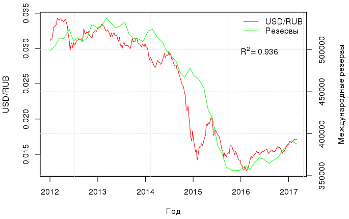
If we construct a linear regression between these two values, then the coefficient of determination will be equal to as much as 0.936. The model with two regressors (oil and reserves) has R ² _adj = 0.98, and, best of all, Ramsey ’s RESET test confirms that there are no missing variables in this regression, i.e. the ruble exchange rate is entirely due to the cost of oil and international reserves:

or, if to scale variables: