Technological stack for classifying natural language texts

In this post we will look at modern approaches used to classify natural language texts according to their topics. The chosen methods of working with documents are determined by the general complex specificity of the task - noisy training samples, samples of insufficient size or no samples at all, a strong distortion of class sizes, and so on. In general - real practical problems. I ask under the cat.

Solvable tasks

There are two main tasks: binary classification and multiclass classification. Binary classification gives us the answer, this document is interesting in general, or it is not at all in the subject and should not be read. Here we have a skewed class size of about 1 to 20, that is - for one good document, there are twenty worthless. But the training sample itself is also problematic - it contains noise both in its completeness and in its accuracy. Noise in terms of completeness is when not all is good, suitable documents are marked as good (FalseNegative), and noise in accuracy - when not all documents marked up as good are actually good (FalsePositive).

The multiclass classification sets us the task of determining the subject of the document and attributing it to one of the hundreds of thematic classes. The training sample for this problem is very noisy in its completeness, but rather pure in accuracy - all the same, the markup is only done manually, not in the first case - on heuristics. But then, thanks to a large number of classes, we begin to enjoy strong distortions in the number of documents per class. The maximum recorded bias is more than 6 thousand. That is, when there is more documents in one class than in the other, 6 thousand times. Just because in the second grade there is one document. Only. But this is not the largest distortion available, since there are classes in which there are zero documents. Well, the assessors did not find the right documents - turn around as you know.

That is, our problems are:
')

• Noisy training samples;
• Severe distortions in class sizes;
• Classes represented by a small number of documents;
• Classes in which there are no documents at all (but you need to work with them).

We will consistently solve these problems by developing one classifier - the signature one, then the other - covering the weak points of the first one - a template, and then we polish it all with machine learning in the form of xgboost and regression. And on top of this ensemble of models we roll a method that covers the shortcomings of all the listed ones - namely, the method of work without training samples in general.

Distributive semantics (Word2Vec)

Google and Yandex know which post to show first when people ask about Word2Vec. Therefore, we will give a brief squeeze from that post and pay attention to what is not written there. Of course, there are other good methods in the distribution semantics section - GloVe, AdaGram, Text2Vec, Seq2Vec, and others. But I didn’t see any strong advantages over W2V in them. If you learn how to work with W2V vectors, you can get amazing results.

Word2Vec:

• It is taught without a teacher on any texts;
• Each token corresponds to a vector of real numbers, such that:
• For any two tokens, you can define the metric * of the distance between them (cosine measure);
• For semantically related tokens, the distance is positive and tends to 1:
• Interchangeable words (Skipgram model);
• Associated words (BagofWords model).

* Not really

Interchangeable words

Enter word or sentence (EXIT to break): coffee

coffe 0.734483
tea 0.690234
tea 0.688656
cappuccino 0.666638
code 0.636362
cocoa 0.619801
espresso 0.599390

Associated words

Enter word or sentence (EXIT to break): coffee

0.757635 grains
soluble 0.709936
tea 0.709579
coffe 0.704036
mellanrost 0.694822
sublimated 0.694553
ground 0.690066
coffee 0.680409

Summarizing a few words (A + B)

Enter word or sentence (EXIT to break): mobile phone

cell 0.811114
phone 0.776416
smartphone 0.730191
telfon 0.719766
mobile 0.717972
mobile phone 0.706131

Projection of Relations (A-B + C)

Find a word that refers to Ukraine as the dollar refers to the United States (that is, what is the currency of Ukraine?):

Enter three words (EXIT to break): us dollar ukraine

UAH 0.622719
Dolar 0.607078
hryvnia 0.597969
Ruble 0.596636

Find such a word that refers to germany as France refers to france (that is, the translation of the word germany):

Enter three words (EXIT to break): france france germany

Germany 0.748171
England 0.692712
Netherlands 0.665715
Great Britain 0.651329

Advantages and disadvantages:

Learning quickly on unprepared texts:

• 1.5 months per 100 GB training file, BagOfWords and Skipgram models, on 24 cores;
• Reduces the dimension:
• 2.5 million tokens dictionary is compressed to 256 elements of the real numbers;
• Vector operations quickly degrade:
• The result of adding 3-5 words is practically useless => not applicable for word processing;

Elements of a vector have no meaning, only the distances between the vectors are meaningful => the metric between the tokens is one-dimensional. This disadvantage is the most offensive. It seems that we already have 256 real numbers, we occupy a whole kilobyte of memory, and in fact the only available operation for us is to compare this vector with another one and get a cosine measure as an estimate of the proximity of these vectors. Process two kilobytes of data, get 4-byte result. And nothing more.

Semantic vector

• The coffee example shows that tokens are grouped by meaning (drinks);
• It is necessary to form a sufficient number of clusters;
• There is no need to mark up the clusters.

Then, we get a set of clusters in which the tokens are grouped by meaning, and, if necessary, each cluster can be assigned the label => each cluster has a meaning independent from the others.
In more detail about the construction of the semantic vector is described in this post .

Text signature

The text consists of tokens, each of which is tied to its cluster;
You can count the number of occurrences of the token in the text and translate into the number of occurrences of the cluster in the text (the sum of all tokens included in the cluster);
Unlike the size of the dictionary (2.5 million tokens), the number of clusters is much less (2048) => the effect of reducing the dimensionality works;

Let's move from the total number of tokens calculated in the text to their relative number (share). Then:

• The share does not depend on the length of the text, but depends only on the frequency of appearance of tokens in the text => it becomes possible to compare texts of different lengths;
• The share characterizes the subject of the text => the subject of the text is determined by the words that are used;

We normalize the proportion of specific texts mat. by expectation and variance calculated over the entire base:

This will increase the importance of rare clusters (not found in all texts - for example, names) as compared with frequent clusters (for example, pronouns, verbs, and other connecting words);

The text is determined by its signature - the vector of 2048 real numbers, meaningful as the normalized shares of the tokens of thematic clusters from which the text is composed.

Signature Classifier

Each text document is assigned a signature;
The tagged training sample of texts turns into the tagged base of signatures;
For the text under study, its signature is formed, which is sequentially compared with the signatures of each file from the training set;
The classification decision is made on the basis of kNN (k nearest neighbors), where k = 3.

Advantages and disadvantages

Benefits:

There is no loss of information from the generalization (comparison is made with each original file from the training sample). The essence of machine learning is to find some patterns, select them and work only with them - drastically reducing the size of the model compared to the size of the training set. True, these are regularities or false ones that have arisen as artifacts of the learning process or because of a lack of training data — it does not matter. The main thing is that the original training information is no longer available - you have to operate only with the model. In the case of a signature-based classifier, we can afford to keep in our memory the entire training sample (not quite so, more on that later - when we talk about classifier tuning). The main thing is that we can determine which particular example from the training set our document looks like the most and connect if necessary an additional analysis of the situation. The lack of generalization is the essence of the absence of loss of information;

Acceptable performance is about 0.3 seconds to run the signature database of 1.7 million documents in 24 streams. And this is without SIMD instructions, but taking into account maximization of cache hits. And in general - dad can in si ;

The ability to highlight fuzzy duplicates:

• Free (comparison of signatures and so happens at the stage of classification);
• High selectivity (only potential duplicates are analyzed, made up mainly of the same tokens, that is, signatures with a high measure of proximity);
• Customizability (you can underestimate the trigger threshold and get not just duplicates, but thematically and stylistically close texts);

Normalization of estimates (0; 1];

The ease of replenishing the training set with new documents (and the ease of excluding documents from it). New training images are connected on the fly - accordingly, the quality of the classifier's performance grows as it works. He is studying. And deleting documents from the database is good for experimenting, building training samples, and so on — just exclude the signature of this particular document from the signature database and run its classification — get a correct assessment of the quality of the classifier's work;

Disadvantages:

The mutual arrangement of tokens (phrases) is not taken into account. It is clear that word combinations are the strongest classifying attribute;
Large minimum requirements for RAM (35+ GB);

Poorly (in no way) does not work when there are a small number of samples per unit. Imagine a 256-dimensional surface of a sphere ... No, it’s better not to. Simply, there is an area in which the documents of our interest should be located. If there are quite a few points in this area — document signatures from the training set — the chances of a new document being close to three of these points are higher (kNN — the same) than if there are proudly 1-2 points in the entire area. Therefore, there are chances to work even with a single positive example per class, but these chances are, of course, not realized as often as we would like.

Accuracy and completeness (binary classification)

How to calculate the score for the binary classification? Very simple - we take the average distance to the 3 best signatures from each class (positive and negative) and evaluate it as:
Positive / (positive + negative).

Therefore, most of the estimates are in a very narrow range, and people, as usual, want to see the numbers interpreted as percentages. That 0.54 is very good, and 0.46 is very bad to explain for a long time and not productively. Still, the graphics look good, classic cross.

Fine-tuning signature classifier

As can be seen from the graph “accuracy and completeness”, the classifier's working area is quite narrow. The solution is to mark up the original text training file that Word2Vec learns from. For this purpose, the labels defining the class of the document are embedded in the document text:

As a result, the clusters are located in the vector space not in a random way, but are divorced so that the clusters of one class will be to each other and stand at a maximum distance from the clusters of the opposite class. Clusters characteristic of both classes are located in the middle.

Memory requirements are reduced by reducing the size of the signature database:

The training sample signatures containing an excessive number of samples (over a million) are sequentially clustered into a large number of clusters, and one signature is used from each cluster. Thereby:

• A relatively uniform coverage of the vector space with sample signatures is preserved;
• Signatures of samples that are too close to each other and, accordingly, are of little use for classification are removed.

Signature classifier, summary

• Fast;
• Easily complemented;
• Allows you to also detect duplicates;
• Does not take into account the mutual arrangement of tokens;
• It does not work when there are few examples in the training set.

Template Classifier

To correct the shortcomings of the signature classifier is designed a classifier on the templates. On ngramma, simply put. If the signature classifier matches the text with the signature and stumbles when there are few such signatures, the template classifier reads the contents of the text more thoughtfully and, if the text is large enough, even a single text is enough to highlight a large number of classifying features.

Template Classifier:

Based on grams up to 16 elements long:

Some target texts are framed according to standards (ISO). There are many typical elements:

• Headers;
• Signatures;
• Coordination sheets and archive tags;

Some of the target documents contain information on registration:

• Xml (including all modern office standards);
• Html;

Almost all contain stable phrases, for example:

• “Strictly confidential, burn before reading”;

Is a simplified implementation of the Naive Baess classifier (without normalization);
Generate up to 60 mln grading grams;
Runs fast (state machine).

Building a classifier

Grams are distinguished from texts;
Calculates the relative frequency of grams per class;
If for different classes the relative frequency is very different (at times), the gram is a classification feature;
Rare grams, met 1 time, are discarded;

The training set is classified, and according to the documents for which the classification was erroneous, additional grams are formed and added to the common gram base.

Classifier use

Grams are distinguished from the text;
Weights of all grams for each class to which they belong are summed;
The class with the highest weights is the winner;
Wherein:

• The class in which there were more teaching texts usually forms more grading grams;
• A rare class (few teaching texts) generates few grams, but their average weight is higher (due to the prevalence of long unique grams for this class);
• The text in which there is no obvious predominance of rare long grams will be assigned to a class with a large number of teaching examples (the posterior distribution tends to a priori). This is how the original naive Baess works and, in general, all universal classifiers;
• A text that has long unique grams of a rare class will be referred rather to this rare class (deliberately introduced distortion in the a posteriori distribution in order to increase selectivity in rare classes). Money pays for the result, and the harder it is to get a result, the more money. It's clear. The most difficult result is just rare thematic classes. Therefore, it makes sense to distort your classifier in such a way that it would be better to look for rare classes, albeit sagging as in large, pop classes. In the end, with the pop classes perfectly handles the signature classifier.

Advantages and disadvantages

Benefits:

• Relatively fast and compact;
• Not bad parallels;
• Able to learn from a single document in a training sample per class;

Disadvantages:

• Estimates are not normalized and, in their original form, do not provide a pairwize criterion (it cannot be guaranteed that a higher weight score is more likely);
• A huge number of grams is generated with a near-zero probability of meeting them in real documents (not duplicates). But then, having met such a rare gram in a document, you can immediately say a lot about this document. And there is enough memory on the server - this is not a problem;
• Huge memory requirements at the training stage. Yes, we need a cluster, but we have them (see poskriptum to this post).

Nonnormalized ratings

Why:

There is no need to do normalization - a strong simplification of the code;
Non-normalized estimates contain more potentially available information for classification.

How to use:

Classifier ratings are good signs for use in universal classifiers (xgboost, SVM, ANN);
At the same time, universal classifiers themselves determine the optimal value of the normalization.

Final generalized classifier (multiclass)

The answers of the signature and template classifiers are combined into a single feature vector, which is subjected to additional processing:

• Normalizing grades to a unit, to get their relative share per class;
• Grouping rare classes to get enough teaching examples per group;
• Taking the difference of group estimates for a flatter surface for gradient descent.

According to the resulting feature vector, the xgboost model is constructed, giving an accuracy gain of up to 3% to the accuracy of the original classifiers.

Binary generalized classifier

Essence of regression from:

• Signature Classifier:
• Template Classifier:
• XgBoost at the outputs of the signature and template classifier.

The optimization criterion is the maximum of the area under the product of completeness and accuracy on the [0; 1] segment; at the same time, issuing a classifier that does not fall into the segment is considered a false positive.

What gives:

Maximizes the classifier work area. Humans see the usual estimate in the form of percentages, from zero to one hundred, at the same time, this estimate falls in such a way as to maximize both completeness and accuracy. It is clear that the maximum of the work is in the area of ​​the cross, where both the completeness and accuracy do not have too small values, but the areas on the right and left, where high completeness is multiplied by no accuracy and where high accuracy is multiplied by no completeness, are uninteresting. No money is paid for them;

Rejects some of the examples to the region below zero => is a signal that the classifier is not able to work out these examples => the classifier fails. From an engineering point of view, this is generally an excellent ability - the classifier himself honestly warns that yes, there are 1-2% of good documents in the discarded stream, but the classifier itself does not know how to work with them - use other methods. Or reconcile.

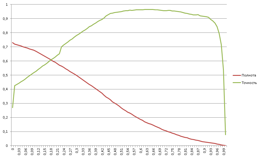
Binary generalized classifier, 1:20

Chic schedule, especially happy blockage on the right. I remind you that here we have a ratio of positive examples in the stream is twenty times less than negative ones. Nevertheless, the graph of completeness looks quite canonical - convex-concave with a knee point in the middle, in the region of 0.3. Why this is important, we show further.

Binary Generalized Classifier, 1:20, Analysis

Completeness begins with 73% => 27% of all positive examples cannot be effectively worked out by the classifier. These 27% of positive examples were in the region below zero precisely because of the optimization of the regression. It is better for business to report that we are not able to work with these documents than to give false negatives to them. But the classifier’s workspace starts with almost 30% accuracy - and these are the numbers that businesses already like;
There is a blockage of accuracy from 96% to 0% => in the sample there are about 4% of examples marked as negative, although in fact they are positive (the problem of completeness of markup);

Five areas are clearly visible:

• Classifier failure area (less than zero);
• two quasilinear regions;
• Saturation region (maximum efficiency);
• Dam area (problem of completeness of markup).

The division into regions makes it possible to develop additional means of classification for each of the regions, especially for the 1st and 5th.

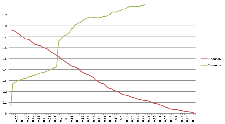
Binary generalized classifier, 1: 182

Here we solve the same problem of binary classification, but at the same time, 182 negative ones fall on one positive example.

Binary Generalized Classifier, 1: 182, Analysis

Completeness begins with 76% => 24% of all positive examples cannot be effectively worked out by the classifier;
12% of all positive examples are clearly recognized by the classifier (100% accuracy);
Four areas are clearly visible:

• Classifier failure area (less than zero);
• two quasilinear regions;
• The area is 100% accurate.

The completeness graph is concave without inflection points => the classifier has a high selectivity (corresponds to the right side of the classical completeness graph with an inflection point in the middle).

Building a classifier for classes that do not have teaching examples

The reality is that there is a sufficiently large number of classes for which no documents have been marked up, and the only information available is the Customer’s message about which documents he wants to classify into this class.

It is impossible to build a training sample manually, since for 1.7 million documents available in the database, only a few documents can be expected to fall under this class, and perhaps not just one.

Class “Marketing research cosmetics”

From the analysis of the class name, we see that the Customer is interested in documents relating to “Marketing Research” and “Cosmetics”. To detect such documents you need:

To form a semantic core of texts on given topics, in this case, in all languages ​​of interest;
Find those topics that are not related to a given class - use them as negative examples (for example, politics);
Find in the database of documents several samples of documents that have a partial or exact relation to a given class;
Mark the found documents by the Assessors of the Customer;
Build a classifier.

Build semantic core texts.

Go to Wikipedia and find an article called, oddly enough, “ marketing research ”. Below there is an inconspicuous reference " category ." In the categories are given all the Wikipedia articles on this topic and nested categories with their articles. In general - a rich source of thematic texts.

But that's not all. On the right in the menu are links to similar articles and categories in other languages. Texts of the same subject, but in languages ​​that interest us. Or on everyone - the classifiers themselves will understand.

Using semantic kernels

We have three themes:

• Marketing research;
• Cosmetics;
• Politics.

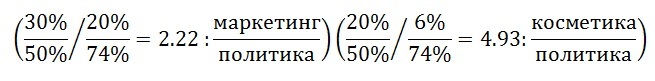
We use the template classifier for these three classes. We will process all documents in the database of documents and get:

• Marketing research 20%;
• Cosmetics 6%;
• Politics 74%.

These shares do not show the actual distribution of documents by subject, they show only the average weights of features of each class, highlighted by the template classifier.

However, if a document is examined that has a distribution of 30%, 20%, 50% shares of such a document, it can be argued that it contains more features of a text with given topics against negative topics (politics), respectively - this text is potentially interesting:

Document Search Results

As a result of processing the entire database of documents, ~ 80 documents were allocated, of which: Two turned out to be fully compliant with the class:

• were not previously found when processing documents manually;
• In different languages ​​other than the entry point into the semantic core (Russian);

~ 36% of all documents found are partially related to the class;
The rest are not related to the class at all.

It is important that as a result of the assessment a marked selection of ~ 80 documents was received, containing both positive and negative examples.

Building a classifier

More than 60% of false positives signal that a single policy is not enough as a negative example.

Decision:

To automatically find other topics of texts that can be used as negative and, potentially, positive examples. For this:

To form automatically sets of texts on a large number of topics and select those that correlate (negatively or positively) with a marked selection of ~ 80 documents.

DBPedia ontology

If someone else does not know, all of Wikipedia is already kindly parsed and laid out in RDF files. Take it and use it. Of interest:

• ShortAbstracts - a brief annotation of the article;
• LongAbstracts - long abstract article;
• Homepages - links to external resources, home pages;
• Article Categories - page category;
• Categorylabels - readable category names;
• Externallinks - links to external resources on the topic;
• Interlanguagelinks - The same article in other languages.

It is worth remembering that DBPedia does not replace Wikipedia as a source of texts for computer linguistics, since the size of the annotation is usually 1-2 paragraphs and cannot be compared with most articles in terms of volume. But no one forbids pumping out your favorite articles and their categories from Wikipedia in the future, right?

[Expected] search results for correlated topics in DBPEdia

The result of the search for correlated topics will be:

• Sets of texts in all languages ​​on specified topics;
• Evaluation of the degree of correlation of texts in relation to the class;
• Human readable (verbal) description of topics.

At the same time, the correlated subjects depend not only on the class “Marketing research of cosmetics”, but also on the topics of the documents contained in the database (for topics with negative correlation). What allows to use the found subjects:

• for manual construction of classifiers on other topics;
• as additional features for texts classified by the final generalized classifier;
• To create additional measurements of similarity metrics in the vector space of the signature classifier: here I refer to my article in the collection of the 2015 Dialogue on learning by analogy in mixed ontological networks. And to the corresponding post .

P.S

This post showed the technologies that we use at the moment and where we plan to move in the future (and these are ontologies). Taking this opportunity, I want to say that in our group we recruit people who are beginning / continuing to study machine linguistics, we are especially glad to see students / graduates who you know which universities.