Open machine learning course. Theme 5. Compositions: bagging, random forest
We will devote the fifth article of the course to simple composition methods: bagging and random forest. You will learn how to get the distribution of the average for the general population, if we have information only about a small part of it; We will see how using composition of algorithms to reduce the variance and thus improve the accuracy of the model; Let us analyze what a random forest is, what parameters it is necessary to “twist” and how to find the most important feature. Let's concentrate in practice by adding a “pinch” of mathematics.
UPD: now the course is in English under the brand mlcourse.ai with articles on Medium, and materials on Kaggle ( Dataset ) and on GitHub .
Video recording of the lecture based on this article in the second run of the open course (September-November 2017).
- Primary data analysis with Pandas
- Visual data analysis with Python
- Classification, decision trees and the method of nearest neighbors
- Linear classification and regression models
- Compositions: bagging, random forest
- Construction and selection of signs
- Teaching without a teacher: PCA, clustering
- Training in gigabytes with Vowpal Wabbit
- Time Series Analysis with Python
- Gradient boosting
Plan for this article
- Bagging
- Random forest
- Assessment of the importance of signs
- Pros and cons of random forest
- Homework number 5
- Useful sources
1. Bagging
From past lectures you have already learned about the different classification algorithms, and also learned how to correctly validate and evaluate the quality of the model. But what if you have already found the best model and can no longer increase the accuracy of the model? In this case, you need to apply more advanced machine learning techniques that can be combined with the word "ensembles". An ensemble is a certain aggregate, parts of which form a single whole. From everyday life, you know musical ensembles, where several musical instruments are combined, architectural ensembles with different buildings, etc.
Ensembles
A good example of ensembles is the Condorcet theorem on the jury (1784). If each member of the jury has an independent opinion, and if the probability of the correct decision of the jury member is more than 0.5, then the probability of the correct decision of the jury as a whole increases with the number of jury members and tends to one. If the probability of being right for each of the jury members is less than 0.5, then the probability of making the right decision by the jury as a whole decreases monotonically and tends to zero with an increase in the number of jurors.
l a r g e N - number of jurors
l a r g e p - the probability of the correct decision of the jury
l a r g e m u - the probability of the correct decision of the entire jury
l a r g e m - the minimum majority of the jury members, m = t e x t f l o o r ( N / 2 ) + 1
l a r g e C i N - number of combinations of N by i
large mu= sumNi=mCiNpi(1−p)N−i
If a largep>0.5 then large mu>p
If a largeN rightarrow infty then large mu rightarrow1
Let's look at another example of ensembles - "The Wisdom of the crowd." In 1906, Francis Galton visited the market, where a certain lottery for peasants was held. 
About 800 people gathered, and they tried to guess the weight of the bull that stood in front of them. The bull weighed 1198 pounds. No peasant guessed the exact weight of the bull, but if you count the average of their predictions, you get 1197 pounds.
This idea of reducing errors was also applied in machine learning.
Bootstrap
Bagging (from Bootstrap aggregation) is one of the first and simplest types of ensembles. It was coined by Leo Brijman in 1994. Bagging is based on the bootstrap statistical method, which allows estimating many statistics of complex distributions.
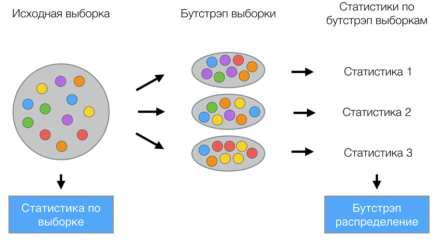
The bootstrap method is as follows. Let there be a sample largeX size largeN . Uniformly take from the sample largeN objects with return. That means we will largeN select an arbitrary sample object (we assume that each object is “picked up” with the same probability large frac1N ), and each time we choose from all the source largeN objects. One can imagine the bag from which the balls are taken: the ball selected at some step returns back to the bag, and the next choice is again made equally probable from the same number of balls. Note that due to the return among them will be repetitions. Denote the new sample by largeX1 . Repeating the procedure largeM times, we will generate largeM subsamples largeX1, dots,XM . Now we have a fairly large number of samples and can evaluate various statistics of the original distribution.
For example, let's take the telecom_churn data set already known to you from the past lessons of our course. Recall that this is the task of binary classification of customer churn. One of the most important signs in this dataset is the number of calls made by the customer to the service center. Let's try to visualize the data and look at the distribution of this trait.
import pandas as pd from matplotlib import pyplot as plt plt.style.use('ggplot') plt.rcParams['figure.figsize'] = 10, 6 import seaborn as sns %matplotlib inline telecom_data = pd.read_csv('data/telecom_churn.csv') fig = sns.kdeplot(telecom_data[telecom_data['Churn'] == False]['Customer service calls'], label = 'Loyal') fig = sns.kdeplot(telecom_data[telecom_data['Churn'] == True]['Customer service calls'], label = 'Churn') fig.set(xlabel=' ', ylabel='') plt.show() 
As you may have noticed, the number of calls to the service center for loyal customers is less than that of our former customers. Now it would be good to estimate how many calls each group makes on average. Since there is little data in our dataset, it’s not quite right to look for the average, it’s better to apply our new bootstrap knowledge. Let's generate 1000 new subsamples from our population and make an interval estimate of the average.
import numpy as np def get_bootstrap_samples(data, n_samples): # indices = np.random.randint(0, len(data), (n_samples, len(data))) samples = data[indices] return samples def stat_intervals(stat, alpha): # boundaries = np.percentile(stat, [100 * alpha / 2., 100 * (1 - alpha / 2.)]) return boundaries # numpy loyal_calls = telecom_data[telecom_data['Churn'] == False]['Customer service calls'].values churn_calls= telecom_data[telecom_data['Churn'] == True]['Customer service calls'].values # seed np.random.seed(0) # loyal_mean_scores = [np.mean(sample) for sample in get_bootstrap_samples(loyal_calls, 1000)] churn_mean_scores = [np.mean(sample) for sample in get_bootstrap_samples(churn_calls, 1000)] # print("Service calls from loyal: mean interval", stat_intervals(loyal_mean_scores, 0.05)) print("Service calls from churn: mean interval", stat_intervals(churn_mean_scores, 0.05)) As a result, we obtained that, with a 95% probability, the average number of calls from loyal customers would lie between 1.40 and 1.50, while our former customers called on average from 2.06 to 2.40 times. You can also note that the interval for loyal customers is already, which is quite logical, since they rarely call (mostly 0, 1 or 2 times), and dissatisfied customers will call much more often, but over time their patience will end, and they will change the operator.
Bagging
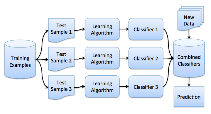
Now you have an idea about boosterp, and we can go directly to bagging. Let there is a training set. largeX . With the help of bootstrap we will generate samples from it. largeX1, dots,XM . Now on each sample we will train your classifier largeai(x) . The final classifier will average the responses of all these algorithms (in the case of classification, this corresponds to a vote): largea(x)= frac1M sumMi=1ai(x) . This scheme can be represented by the picture below.
Consider a regression problem with basic algorithms. largeb1(x), dots,bn(x) . Suppose there is a true answer function for all objects largey(x) , and also set the distribution on objects largep(x) . In this case, we can write the error of each regression function.
large varepsiloni(x)=bi(x)−y(x),i=1, dots,n
and write the expectation of the standard error
largeEx(bi(x)−y(x))2=Ex varepsilon2i(x).
The average error of the constructed regression functions is
largeE1= frac1nEx sumni=1 varepsilon2i(x)
Suppose the errors are unbiased and uncorrelated:
\ large \ begin {array} {rcl} E_x \ varepsilon_i (x) & = & 0, \\ E_x \ varepsilon_i (x) \ varepsilon_j (x) & = & 0, i \ neq j. \ end {array}
We now build a new regression function that will average the responses of the functions we have constructed:
largea(x)= frac1n sumni=1bi(x)
Find its root-mean-square error:
\ large \ begin {array} {rcl} E_n & = & E_x \ Big (\ frac {1} {n} \ sum_ {i = 1} ^ {n} b_i (x) -y (x) \ Big) ^ 2 \\ & = & E_x \ Big (\ frac {1} {n} \ sum_ {i = 1} ^ {n} \ varepsilon_i \ Big) ^ 2 \\ & = & \ frac {1} {n ^ 2} E_x \ Big (\ sum_ {i = 1} ^ {n} \ varepsilon_i ^ 2 (x) + \ sum_ {i \ neq j} \ varepsilon_i (x) \ varepsilon_j (x) \ Big) \\ & = & \ frac {1} {n} E_1 \ end {array}
Thus, averaging the answers allowed to reduce the average square of the error by n times!
Let us remind you from our previous lesson how the general error is decomposed:
\ large \ begin {array} {rcl} \ text {Err} \ left (\ vec {x} \ right) & = & \ mathbb {E} \ left [\ left (y - \ hat {f} \ left (\ vec {x} \ right) \ right) ^ 2 \ right] \\ & = & \ sigma ^ 2 + f ^ 2 + \ text {Var} \ left (\ hat {f} \ right) + \ mathbb {E} \ left [\ hat {f} \ right] ^ 2 - 2f \ mathbb {E} \ left [\ hat {f} \ right] \\ & = & \ left (f - \ mathbb {E} \ left [\ hat {f} \ right] \ right) ^ 2 + \ text {Var} \ left (\ hat {f} \ right) + \ sigma ^ 2 \\ & = & \ text {Bias} \ left ( \ hat {f} \ right) ^ 2 + \ text {Var} \ left (\ hat {f} \ right) + \ sigma ^ 2 \ end {array}
Bagging allows you to reduce the variance of a trained classifier, reducing the amount by which the error will differ if you train the model on different data sets, or in other words, it prevents retraining. The effectiveness of bagging is achieved due to the fact that the basic algorithms trained in various subsamples are quite different, and their errors are mutually compensated for when voting, and also due to the fact that emission objects may not fall into some of the training subsamples.
In the scikit-learn library, there are BaggingRegressor and BaggingClassifier implementations that allow you to use most other algorithms "inside". Let us consider in practice how bagging works, and compare it with the decision tree, using the example from the documentation .

Decision Tree Error
large0.0255(Err)=0.0003(Bias2)+0.0152(Var)+0.0098( sigma2)
Bugging error
large0.0196(Err)=0.0004(Bias2)+0.0092(Var)+0.0098( sigma2)
The graph and the results above show that the variance error is much smaller during bagging, as we proved theoretically higher.
Bagging is effective on small samples, when the exclusion of even a small part of the training objects leads to the construction of substantially different basic classifiers. In the case of large samples, subsamples are usually generated that are significantly shorter.
It should be noted that the example we have considered is not very applicable in practice, since we made the assumption that errors are not correlated, which is rarely done. If this assumption is wrong, then the error reduction is not so significant. In the following lectures, we will consider more complex methods of combining algorithms into a composition that allow us to achieve high quality in real-world problems.
Out-of-bag error
Looking ahead, we note that when using random forests there is no need for cross-validation or in a separate test set to get an unbiased error estimate for the test suite. Let's see how it turns out the "internal" assessment of the model during its training.
Each tree is built using different bootstrap samples from the source data. Approximately 37% of the examples remain outside the bootstrap sample and are not used when building the kth tree.
This can be easily proved: let in the sample large ell objects. At each step, all objects fall into a subsample with return equiprobably, that is, a separate object with probability large frac1 ell. The probability that an object will NOT fall into a subsample (i.e. it was not taken large ell time): large(1− frac1 ell) ell . With large ell rightarrow+ infty we get one of the "wonderful" limits large frac1e . Then the probability of hitting a particular object in the subsample large approx1− frac1e approx63% .
Let's look at how this works in practice:
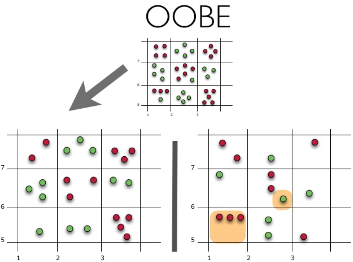
The figure shows the oob error estimate. The top figure is our original sample, we divide it into a training one (left) and a test one (right). In the picture to the left, we have a grid of squares, which ideally breaks our sample. Now we need to estimate the proportion of correct answers on our test sample. The figure shows that our classifier made a mistake in 4 observations that we did not use for training. Hence, the proportion of correct answers of our classifier: large frac1115∗100%=73.33%
It turns out that each basic algorithm is trained on ~ 63% of the original objects. This means that it can be immediately checked for the remaining ~ 37%. Out-of-Bag estimation is the average estimate of the basic algorithms for those ~ 37% of the data on which they were not trained.
2. Random forest
Leo Breyman found the use of bootstrap not only in statistics, but also in machine learning. He, along with Adel Cutler, improved the random forest algorithm proposed by Ho , adding to the original version the construction of uncorrelated trees based on CART, in combination with the method of random subspaces and bagging.
Decisive trees are a good family of basic classifiers for bagging, since they are quite complex and can reach zero error on any sample. The method of random subspaces allows to reduce the correlation between trees and to avoid retraining. Basic algorithms are trained on different subsets of the feature description, which are also randomly selected.
An ensemble of models using the random subspace method can be constructed using the following algorithm:
- Let the number of objects for learning be largeN , and the number of signs largeD .
- Select largeL as the number of individual models in the ensemble.
- For each individual model largel select largedl(dl<D) as the number of signs for largel . Usually for all models only one value is used. largedl .
- For each individual model largel create a training set by selecting largedl signs of largeD and train the model.
- Now, to apply the ensemble model to a new object, combine the results of the individual largeL majority voting models or by combining a posteriori probabilities.
Algorithm
The algorithm for constructing a random forest consisting of largeN trees, looks like this:
- For each largen=1, dots,N :
- Generate a sample largeXn using bootstrap;
- Build a decisive tree largebn by sample largeXn :
- according to a given criterion, we choose the best attribute, make a split in the tree according to it, and so on until the sample is exhausted
- the tree is built, while in each sheet no more largen textmin objects or until you reach a certain tree height
- at each splitting, first selected largem random signs from largen source,
and the optimal sampling separation is sought only among them.
Final Classifier largea(x)= frac1N sumNi=1bi(x) , in simple words - for the problem of cassification we choose the solution by voting on the majority, and in the regression problem - on the average.
It is recommended to take in classification tasks largem= sqrtn , and in regression problems - largem= fracn3 where largen - the number of signs. It is also recommended to build each tree in the classification tasks until there is one object in each sheet, and in regression problems, until five objects are in each sheet.
Thus, a random forest is a bugging over the decisive trees, when training them, for each partition, the signs are selected from some random subset of features.
Comparison with decision tree and bagging
from __future__ import division, print_function # Anaconda import warnings warnings.filterwarnings('ignore') %pylab inline np.random.seed(42) figsize(8, 6) import seaborn as sns from sklearn.ensemble import RandomForestRegressor, RandomForestClassifier, BaggingRegressor from sklearn.tree import DecisionTreeRegressor, DecisionTreeClassifier n_train = 150 n_test = 1000 noise = 0.1 # Generate data def f(x): x = x.ravel() return np.exp(-x ** 2) + 1.5 * np.exp(-(x - 2) ** 2) def generate(n_samples, noise): X = np.random.rand(n_samples) * 10 - 5 X = np.sort(X).ravel() y = np.exp(-X ** 2) + 1.5 * np.exp(-(X - 2) ** 2)\ + np.random.normal(0.0, noise, n_samples) X = X.reshape((n_samples, 1)) return X, y X_train, y_train = generate(n_samples=n_train, noise=noise) X_test, y_test = generate(n_samples=n_test, noise=noise) # One decision tree regressor dtree = DecisionTreeRegressor().fit(X_train, y_train) d_predict = dtree.predict(X_test) plt.figure(figsize=(10, 6)) plt.plot(X_test, f(X_test), "b") plt.scatter(X_train, y_train, c="b", s=20) plt.plot(X_test, d_predict, "g", lw=2) plt.xlim([-5, 5]) plt.title(" , MSE = %.2f" % np.sum((y_test - d_predict) ** 2)) # Bagging decision tree regressor bdt = BaggingRegressor(DecisionTreeRegressor()).fit(X_train, y_train) bdt_predict = bdt.predict(X_test) plt.figure(figsize=(10, 6)) plt.plot(X_test, f(X_test), "b") plt.scatter(X_train, y_train, c="b", s=20) plt.plot(X_test, bdt_predict, "y", lw=2) plt.xlim([-5, 5]) plt.title(" , MSE = %.2f" % np.sum((y_test - bdt_predict) ** 2)); # Random Forest rf = RandomForestRegressor(n_estimators=10).fit(X_train, y_train) rf_predict = rf.predict(X_test) plt.figure(figsize=(10, 6)) plt.plot(X_test, f(X_test), "b") plt.scatter(X_train, y_train, c="b", s=20) plt.plot(X_test, rf_predict, "r", lw=2) plt.xlim([-5, 5]) plt.title(" , MSE = %.2f" % np.sum((y_test - rf_predict) ** 2)); 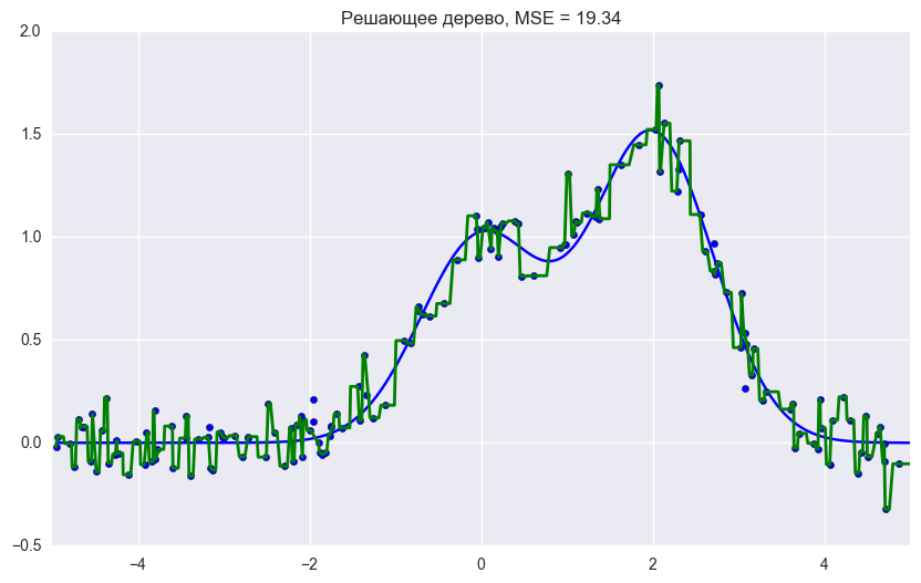


As we can see from the graphs and MSE error values, a random forest of 10 trees gives a better result than a single tree or bagging of 10 decision trees. The main difference between random forest and bagging on decision trees is that a random subset of features is selected in a random forest, and the best attribute for separating a node is determined from a subsample of attributes, unlike bagging, where all functions are considered for separation in a node.
You can also see the advantage of random forest and bagging in classification tasks.
from sklearn.ensemble import RandomForestClassifier, BaggingClassifier from sklearn.tree import DecisionTreeClassifier from sklearn.datasets import make_circles from sklearn.cross_validation import train_test_split import numpy as np from matplotlib import pyplot as plt plt.style.use('ggplot') plt.rcParams['figure.figsize'] = 10, 6 %matplotlib inline np.random.seed(42) X, y = make_circles(n_samples=500, factor=0.1, noise=0.35, random_state=42) X_train_circles, X_test_circles, y_train_circles, y_test_circles = train_test_split(X, y, test_size=0.2) dtree = DecisionTreeClassifier(random_state=42) dtree.fit(X_train_circles, y_train_circles) x_range = np.linspace(X.min(), X.max(), 100) xx1, xx2 = np.meshgrid(x_range, x_range) y_hat = dtree.predict(np.c_[xx1.ravel(), xx2.ravel()]) y_hat = y_hat.reshape(xx1.shape) plt.contourf(xx1, xx2, y_hat, alpha=0.2) plt.scatter(X[:,0], X[:,1], c=y, cmap='autumn') plt.title(" ") plt.show() b_dtree = BaggingClassifier(DecisionTreeClassifier(),n_estimators=300, random_state=42) b_dtree.fit(X_train_circles, y_train_circles) x_range = np.linspace(X.min(), X.max(), 100) xx1, xx2 = np.meshgrid(x_range, x_range) y_hat = b_dtree.predict(np.c_[xx1.ravel(), xx2.ravel()]) y_hat = y_hat.reshape(xx1.shape) plt.contourf(xx1, xx2, y_hat, alpha=0.2) plt.scatter(X[:,0], X[:,1], c=y, cmap='autumn') plt.title("( )") plt.show() rf = RandomForestClassifier(n_estimators=300, random_state=42) rf.fit(X_train_circles, y_train_circles) x_range = np.linspace(X.min(), X.max(), 100) xx1, xx2 = np.meshgrid(x_range, x_range) y_hat = rf.predict(np.c_[xx1.ravel(), xx2.ravel()]) y_hat = y_hat.reshape(xx1.shape) plt.contourf(xx1, xx2, y_hat, alpha=0.2) plt.scatter(X[:,0], X[:,1], c=y, cmap='autumn') plt.title(" ") plt.show() 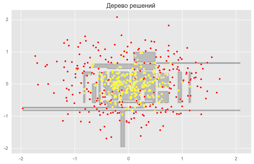
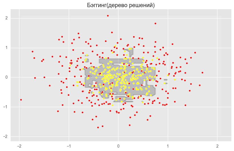
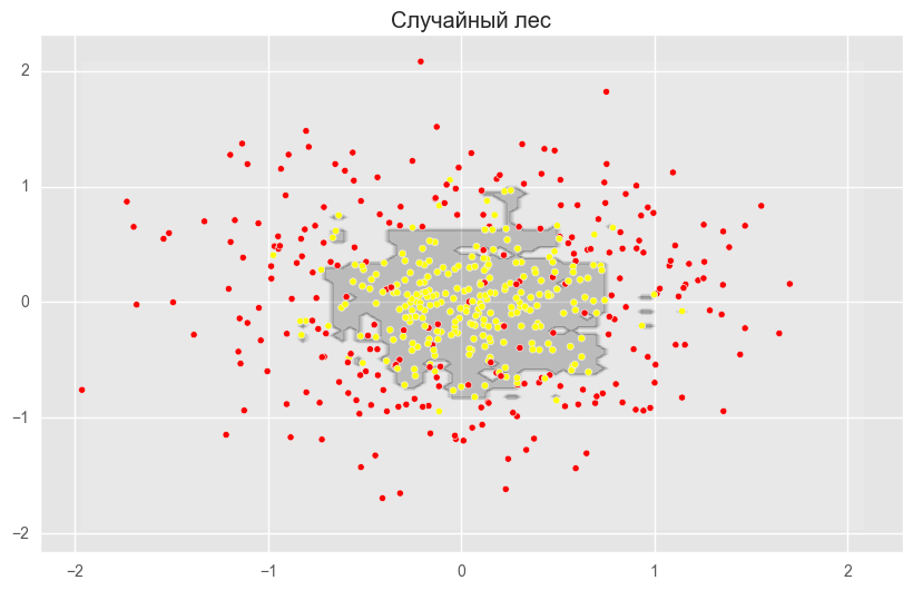
The figures above show that the dividing boundary of the decision tree is very “ragged” and there are a lot of sharp corners on it, which indicates retraining and weak generalizing ability. While in bagging and random forest, the border is rather smooth and there are almost no signs of retraining.
Let's now try to figure out the parameters, by choosing which we can increase the proportion of correct answers.
Options
The random forest method is implemented in the scikit-learn machine learning library with two classes: RandomForestClassifier and RandomForestRegressor.
A complete list of random forest parameters for the regression problem:
class sklearn.ensemble.RandomForestRegressor( n_estimators — "" ( – 10) criterion — , ( — "mse" , "mae") max_features — , . , : "auto" ( ), "sqrt", "log2". "auto". max_depth — ( ) min_samples_split — , . ( — 2) min_samples_leaf — . ( — 1) min_weight_fraction_leaf — ( ) ( ) max_leaf_nodes — ( ) min_impurity_split — ( 1-7) bootstrap — ( True) oob_score — out-of-bag R^2 ( False) n_jobs — ( 1, -1, ) random_state — ( , , int verbose — ( 0) warm_start — ( False) ) For the classification task, everything is almost the same; we will only list the parameters by which RandomForestClassifier differs from RandomForestRegressor.
class sklearn.ensemble.RandomForestClassifier( criterion — , "gini" ( "entropy") class_weight — ( 1, , "balanced", ; "balanced_subsample", . ) Next, we consider several parameters, which, first of all, should be paid attention to when building a model:
- n_estimators - the number of trees in the "forest"
- criterion - criterion for splitting a sample at the vertex
- max_features - the number of features by which the partition is searched.
- min_samples_leaf - the minimum number of objects in the sheet
- max_depth - maximum tree depth
Consider the use of a random forest in a real problem.
For this we will use the example with the problem of churn clients. This is a classification task, so we will use the accuracy metric to assess the quality of the model. To begin with, let's build the simplest classifier that will be our baseline. Take only numeric characters for simplicity.
import pandas as pd from sklearn.model_selection import cross_val_score, StratifiedKFold, GridSearchCV from sklearn.metrics import accuracy_score # df = pd.read_csv("../../data/telecom_churn.csv") # cols = [] for i in df.columns: if (df[i].dtype == "float64") or (df[i].dtype == 'int64'): cols.append(i) # X, y = df[cols].copy(), np.asarray(df["Churn"],dtype='int8') # skf = StratifiedKFold(n_splits=5, shuffle=True, random_state=42) # rfc = RandomForestClassifier(random_state=42, n_jobs=-1, oob_score=True) # results = cross_val_score(rfc, X, y, cv=skf) # print("CV accuracy score: {:.2f}%".format(results.mean()*100)) 91.21%, , .
:
# skf = StratifiedKFold(n_splits=5, shuffle=True, random_state=42) # train_acc = [] test_acc = [] temp_train_acc = [] temp_test_acc = [] trees_grid = [5, 10, 15, 20, 30, 50, 75, 100] # for ntrees in trees_grid: rfc = RandomForestClassifier(n_estimators=ntrees, random_state=42, n_jobs=-1, oob_score=True) temp_train_acc = [] temp_test_acc = [] for train_index, test_index in skf.split(X, y): X_train, X_test = X.iloc[train_index], X.iloc[test_index] y_train, y_test = y[train_index], y[test_index] rfc.fit(X_train, y_train) temp_train_acc.append(rfc.score(X_train, y_train)) temp_test_acc.append(rfc.score(X_test, y_test)) train_acc.append(temp_train_acc) test_acc.append(temp_test_acc) train_acc, test_acc = np.asarray(train_acc), np.asarray(test_acc) print("Best accuracy on CV is {:.2f}% with {} trees".format(max(test_acc.mean(axis=1))*100, trees_grid[np.argmax(test_acc.mean(axis=1))])) import matplotlib.pyplot as plt plt.style.use('ggplot') %matplotlib inline fig, ax = plt.subplots(figsize=(8, 4)) ax.plot(trees_grid, train_acc.mean(axis=1), alpha=0.5, color='blue', label='train') ax.plot(trees_grid, test_acc.mean(axis=1), alpha=0.5, color='red', label='cv') ax.fill_between(trees_grid, test_acc.mean(axis=1) - test_acc.std(axis=1), test_acc.mean(axis=1) + test_acc.std(axis=1), color='#888888', alpha=0.4) ax.fill_between(trees_grid, test_acc.mean(axis=1) - 2*test_acc.std(axis=1), test_acc.mean(axis=1) + 2*test_acc.std(axis=1), color='#888888', alpha=0.2) ax.legend(loc='best') ax.set_ylim([0.88,1.02]) ax.set_ylabel("Accuracy") ax.set_xlabel("N_estimators") 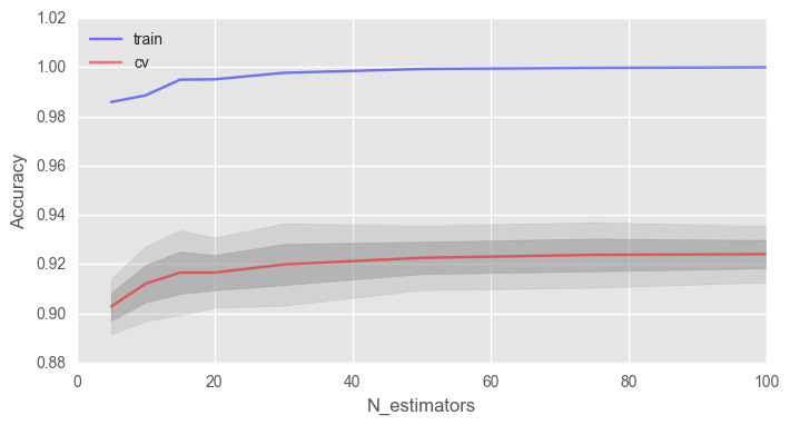
, , , .
, 100% , . , .
– max_depth . ( - 100)
# train_acc = [] test_acc = [] temp_train_acc = [] temp_test_acc = [] max_depth_grid = [3, 5, 7, 9, 11, 13, 15, 17, 20, 22, 24] # for max_depth in max_depth_grid: rfc = RandomForestClassifier(n_estimators=100, random_state=42, n_jobs=-1, oob_score=True, max_depth=max_depth) temp_train_acc = [] temp_test_acc = [] for train_index, test_index in skf.split(X, y): X_train, X_test = X.iloc[train_index], X.iloc[test_index] y_train, y_test = y[train_index], y[test_index] rfc.fit(X_train, y_train) temp_train_acc.append(rfc.score(X_train, y_train)) temp_test_acc.append(rfc.score(X_test, y_test)) train_acc.append(temp_train_acc) test_acc.append(temp_test_acc) train_acc, test_acc = np.asarray(train_acc), np.asarray(test_acc) print("Best accuracy on CV is {:.2f}% with {} max_depth".format(max(test_acc.mean(axis=1))*100, max_depth_grid[np.argmax(test_acc.mean(axis=1))])) fig, ax = plt.subplots(figsize=(8, 4)) ax.plot(max_depth_grid, train_acc.mean(axis=1), alpha=0.5, color='blue', label='train') ax.plot(max_depth_grid, test_acc.mean(axis=1), alpha=0.5, color='red', label='cv') ax.fill_between(max_depth_grid, test_acc.mean(axis=1) - test_acc.std(axis=1), test_acc.mean(axis=1) + test_acc.std(axis=1), color='#888888', alpha=0.4) ax.fill_between(max_depth_grid, test_acc.mean(axis=1) - 2*test_acc.std(axis=1), test_acc.mean(axis=1) + 2*test_acc.std(axis=1), color='#888888', alpha=0.2) ax.legend(loc='best') ax.set_ylim([0.88,1.02]) ax.set_ylabel("Accuracy") ax.set_xlabel("Max_depth") 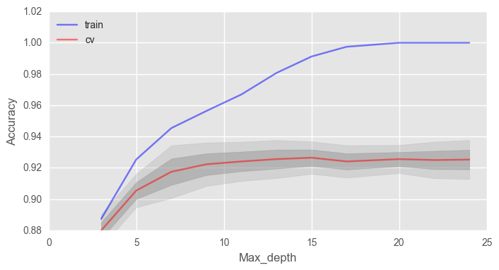
max_depth , . .
min_samples_leaf , .
# train_acc = [] test_acc = [] temp_train_acc = [] temp_test_acc = [] min_samples_leaf_grid = [1, 3, 5, 7, 9, 11, 13, 15, 17, 20, 22, 24] # for min_samples_leaf in min_samples_leaf_grid: rfc = RandomForestClassifier(n_estimators=100, random_state=42, n_jobs=-1, oob_score=True, min_samples_leaf=min_samples_leaf) temp_train_acc = [] temp_test_acc = [] for train_index, test_index in skf.split(X, y): X_train, X_test = X.iloc[train_index], X.iloc[test_index] y_train, y_test = y[train_index], y[test_index] rfc.fit(X_train, y_train) temp_train_acc.append(rfc.score(X_train, y_train)) temp_test_acc.append(rfc.score(X_test, y_test)) train_acc.append(temp_train_acc) test_acc.append(temp_test_acc) train_acc, test_acc = np.asarray(train_acc), np.asarray(test_acc) print("Best accuracy on CV is {:.2f}% with {} min_samples_leaf".format(max(test_acc.mean(axis=1))*100, min_samples_leaf_grid[np.argmax(test_acc.mean(axis=1))])) fig, ax = plt.subplots(figsize=(8, 4)) ax.plot(min_samples_leaf_grid, train_acc.mean(axis=1), alpha=0.5, color='blue', label='train') ax.plot(min_samples_leaf_grid, test_acc.mean(axis=1), alpha=0.5, color='red', label='cv') ax.fill_between(min_samples_leaf_grid, test_acc.mean(axis=1) - test_acc.std(axis=1), test_acc.mean(axis=1) + test_acc.std(axis=1), color='#888888', alpha=0.4) ax.fill_between(min_samples_leaf_grid, test_acc.mean(axis=1) - 2*test_acc.std(axis=1), test_acc.mean(axis=1) + 2*test_acc.std(axis=1), color='#888888', alpha=0.2) ax.legend(loc='best') ax.set_ylim([0.88,1.02]) ax.set_ylabel("Accuracy") ax.set_xlabel("Min_samples_leaf") 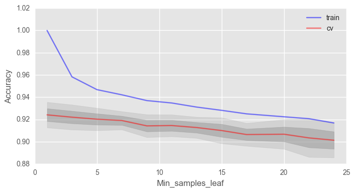
, 2% 92%.
max_features . √n , n — . , 4 .
# train_acc = [] test_acc = [] temp_train_acc = [] temp_test_acc = [] max_features_grid = [2, 4, 6, 8, 10, 12, 14, 16] # for max_features in max_features_grid: rfc = RandomForestClassifier(n_estimators=100, random_state=42, n_jobs=-1, oob_score=True, max_features=max_features) temp_train_acc = [] temp_test_acc = [] for train_index, test_index in skf.split(X, y): X_train, X_test = X.iloc[train_index], X.iloc[test_index] y_train, y_test = y[train_index], y[test_index] rfc.fit(X_train, y_train) temp_train_acc.append(rfc.score(X_train, y_train)) temp_test_acc.append(rfc.score(X_test, y_test)) train_acc.append(temp_train_acc) test_acc.append(temp_test_acc) train_acc, test_acc = np.asarray(train_acc), np.asarray(test_acc) print("Best accuracy on CV is {:.2f}% with {} max_features".format(max(test_acc.mean(axis=1))*100, max_features_grid[np.argmax(test_acc.mean(axis=1))])) fig, ax = plt.subplots(figsize=(8, 4)) ax.plot(max_features_grid, train_acc.mean(axis=1), alpha=0.5, color='blue', label='train') ax.plot(max_features_grid, test_acc.mean(axis=1), alpha=0.5, color='red', label='cv') ax.fill_between(max_features_grid, test_acc.mean(axis=1) - test_acc.std(axis=1), test_acc.mean(axis=1) + test_acc.std(axis=1), color='#888888', alpha=0.4) ax.fill_between(max_features_grid, test_acc.mean(axis=1) - 2*test_acc.std(axis=1), test_acc.mean(axis=1) + 2*test_acc.std(axis=1), color='#888888', alpha=0.2) ax.legend(loc='best') ax.set_ylim([0.88,1.02]) ax.set_ylabel("Accuracy") ax.set_xlabel("Max_features") 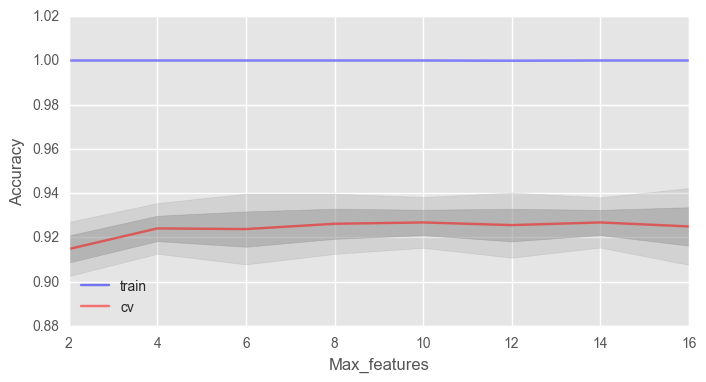
— 10, .
We looked at how the validation curves behave depending on changes in the basic parameters. Let us now with the help GridSearchCVfind the optimal parameters for our example.
# , parameters = {'max_features': [4, 7, 10, 13], 'min_samples_leaf': [1, 3, 5, 7], 'max_depth': [5,10,15,20]} rfc = RandomForestClassifier(n_estimators=100, random_state=42, n_jobs=-1, oob_score=True) gcv = GridSearchCV(rfc, parameters, n_jobs=-1, cv=skf, verbose=1) gcv.fit(X, y) The best proportion of correct answers, which we were able to achieve with the help of the parameter search - 92.83% with 'max_depth': 15, 'max_features': 7, 'min_samples_leaf': 3.
Variation and decorrelation effect
Let's write the variance for a random forest as
V a r f ( x ) = ρ ( x ) σ 2 ( x )
Here
- ρ ( x ) is the sampling correlation between any two trees used in averaging
ρ(x)=corr[T(x;Θ1(Z)),T(x2,Θ2(Z))],
Where Θ1(Z) and Θ2(Z) – Z
σ2(x) — :σ2(x)=VarT(x;Θ(X)
')ρ(X) , N- . . , x at ρ(x) . ρ(x) , x , Z , . , Z and Θ .
, 0, — .
, ( m ), , , .
The Elements of Statistical Learning (Trevor Hastie, Robert Tibshirani Jerome Friedman) , .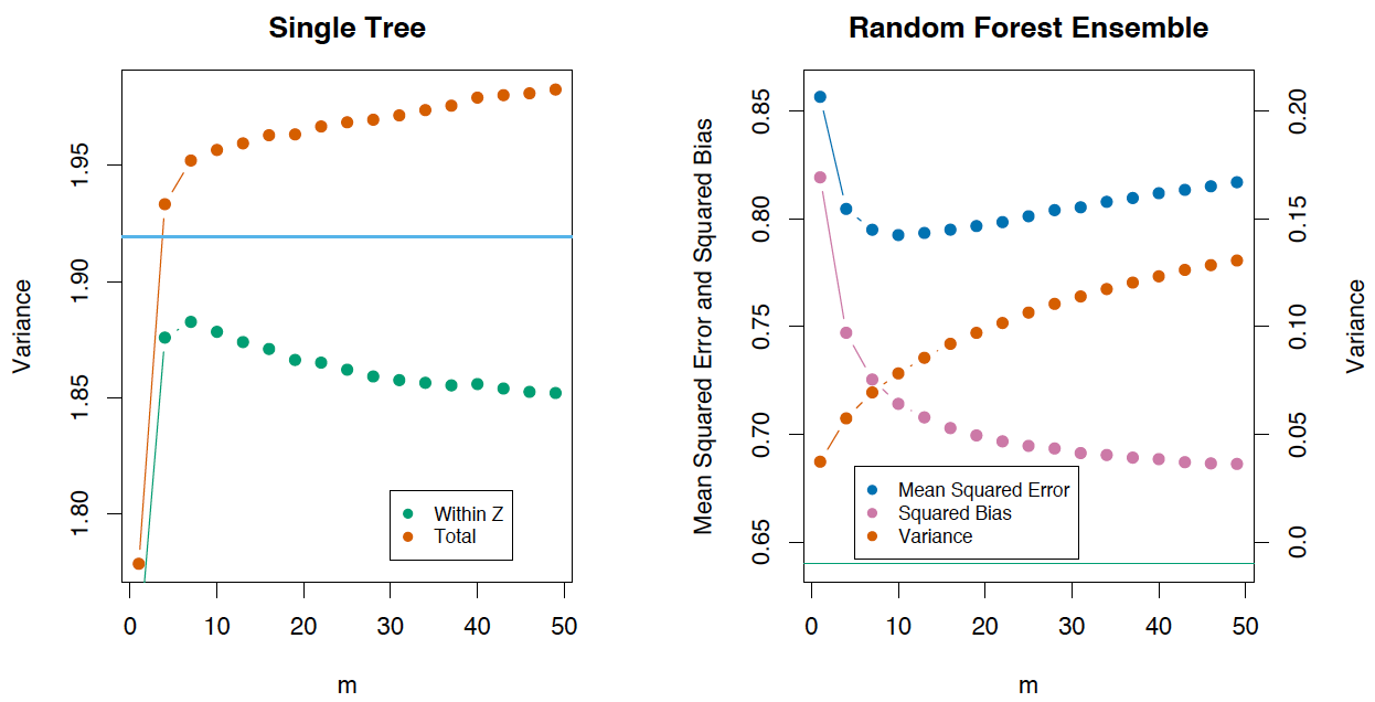
, , T(x,Θ(Z)) :
Bias=μ(x)−EZfrf(x)=μ(x)−EZEΘ|ZT(x,Θ(Z))
( ), «» (unprunned) , . , , , .
(Extremely Randomized Trees) , . , , , , . .
scikit-learn ExtraTreesClassifier ExtraTreesRegressor . , .
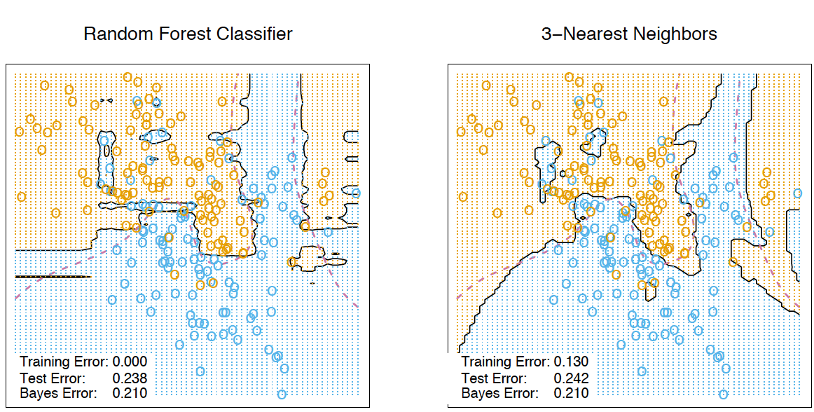
k-
. , , . , . .
. Let be Tn(x) — n(x) - , x . x , Tn(x) .
bn(x)=l∑i=1wn(x,xi)yi,
Where
wn(x,xi)=[Tn(x)=Tn(xi)]∑lj=1[Tn(x)=Tn(xj)]
an(x)=1N∑Nn=1∑li=1wn(x,xi)yi=∑li=1(1N∑Nj=1wn(x,xj))yi
, . , Tn(x) , , . , , T1(x),…,Tn(x) . .The Elements of Statistical Learning k- .
, . RandomTreesEmbedding . , , , , . , 1, , 0. . / . , , .
3.
, , . , . .
The essence of the method
, «» , «». .

( ), , /. ( (Gini impurity)) — , , .
. , , out-of-bag . - ( ) , , ́ . ( mse ) , . , , . 0 () 1 (). . , , .
.
VIT=∑i∈BTI(yi=ˆyTi)|BT|−∑i∈BTI(yi=ˆyTi,πj)|BT|
ˆy(T)i=fT(xi) — /
ˆy(T)i,πj=fT(xi,πj) — /
xi,πj=(xi,1,…,xi,j−1,xπj(i),j,xi,j+1,…,xi,p)
, VI(T)(xj)=0 , Xj T:
—VI(xj)=∑NT=1VIT(xj)N
—
zj=VI(xj)ˆσ√N
Example
Booking.com TripAdvisor.com. — ( ) — , .. — .
from __future__ import division, print_function # Anaconda import warnings warnings.filterwarnings('ignore') %pylab inline import seaborn as sns # russian headres from matplotlib import rc font = {'family': 'Verdana', 'weight': 'normal'} rc('font', **font) import pandas as pd import numpy as np from sklearn.ensemble.forest import RandomForestRegressor hostel_data = pd.read_csv("../../data/hostel_factors.csv") features = {"f1":u"", "f2":u" ", "f3":u" ", "f4":u" ", "f5":u" ", "f6":u" ", "f7":u" ", "f8":u" ", "f9":u"/", "f10":u""} forest = RandomForestRegressor(n_estimators=1000, max_features=10, random_state=0) forest.fit(hostel_data.drop(['hostel', 'rating'], axis=1), hostel_data['rating']) importances = forest.feature_importances_ indices = np.argsort(importances)[::-1] # Plot the feature importancies of the forest num_to_plot = 10 feature_indices = [ind+1 for ind in indices[:num_to_plot]] # Print the feature ranking print("Feature ranking:") for f in range(num_to_plot): print("%d. %s %f " % (f + 1, features["f"+str(feature_indices[f])], importances[indices[f]])) plt.figure(figsize=(15,5)) plt.title(u" ") bars = plt.bar(range(num_to_plot), importances[indices[:num_to_plot]], color=([str(i/float(num_to_plot+1)) for i in range(num_to_plot)]), align="center") ticks = plt.xticks(range(num_to_plot), feature_indices) plt.xlim([-1, num_to_plot]) plt.legend(bars, [u''.join(features["f"+str(i)]) for i in feature_indices]);
, / . , - . / .4.
Pros :
— , ;
— -
— ( ) ,
— , « ». «» 0.5 3%
—
— ,
— , , , ,
—
— ; ,
— ,
— , , ( )
— , , , ,
— .Cons :
— ,
— (p-values),
— , (, Bag of words)
— , ( , )
— ,
— , , : , , ( )
— , ,
— . Is required O(NK) , K — .5.
– . - ( ).
6.
– Open Machine Learning Course. Topic 5. Bagging and Random Forest ( )
–
– 15 “ Elements of Statistical Learning ” Jerome H. Friedman, Robert Tibshirani, and Trevor Hastie
–
– - scikit-learn
– ( GitHub).
– " " (. )yorko ( ). – vradchenko ( ). bauchgefuehl ( ) .
Source: https://habr.com/ru/post/324402/
All Articles