How to search for patterns in stock data and use them in trading?

Today I propose to reflect on how to look for patterns in stock data and how to use them for successful trading.

We will receive Forex exchange data from one of the brokers, save it to the PostgreSQL database and try to find patterns using machine learning algorithms.

The article has some nice bonuses in the form of Python code - you can analyze any (almost) stock data (or indicator values) yourself, run your own trading robot and test any trading strategy.
')
All the conditions and definitions of patterns in the article are for example, you can use any criteria.

What is a pattern and how to use it?

A pattern is a stable, repetitive pattern of consecutive stock data, after the occurrence of which the price is likely to change in the right direction.

Analyzing statistics in order to find repetitive patterns is not an easy task, but if dependencies can be found, then the price movement can be predicted quite accurately. Using the methods of machine learning, the search for patterns comes down to choosing the best classifier - an algorithm that learns from historical data and predicts price movement with a certain probability.

Such a mechanism may well become part of a successful trading strategy in combination with other methods of market analysis.

Training

1. In order to receive historical data and submit applications for Forex through the RESTv20 API, we will need a demo account from a well-known broker . Registration takes a minute, after which you get token (a unique key for access) and account number.
2. Python version 2.7 with installed libraries is required: oandapyV20, sklearn, matplotlib, numpy, psycopg2. They can be installed via pip.
   
3. PostgreSQL is required, I have version 9.6.
   

Model Description

The very first thing to describe is the historical data itself.

Create a class Candle, which will store information about each candle:

class Candle: def __init__(self, datetime, ask, bid, volume): self.datetime = datetime self.ask = ask self.bid = bid self.volume = volume 

The description of the pattern will be as follows:

 class Pattern: result = '' serie = list() def __init__(self, serie, result): self.serie = serie self.result = result 

Each series of data will correspond to the result, in our case, the purchase or sale.
Here you need to not forget that we are interested in the form . This means that it is not true to describe the pattern simply by prices, their normalization is necessary. About this below.

We introduce two more parameters:

1. Series length ( Length ) - the number of consecutive elements in the pattern series
2. Window width ( window size) - the number of consecutive elements after the series, for at least one of which the condition for choosing a pattern is met

What are the conditions for choosing patterns ? - so as to make a profit:

If we buy at the ask = X price, then we should sell at the increased bid > X price. And vice versa, if we sell at the bid = Y price, then we should buy at the ask <Y price. In this, the price change will be greater than the spread at the time of purchase and we will make a profit.
Today I propose to use these simple rules for selecting patterns, but in fact, in order for everything to work well, you need to add a few filters to them. I suggest that you do it yourself later. Do not forget that the choice of source data (period, market, instrument, etc.) is very important - somewhere there are patterns, and somewhere there are not. Or you need to change the conditions of their selection.

Get the data

We will receive data from the broker and save it in the PostgreSQL database. First of all, let's create a class that will load data:

 import pandas from oandapyV20.endpoints import instruments class StockDataDownloader(object): def get_data_from_finam(self, ticker, period, marketCode, insCode, dateFrom, dateTo): """Downloads data from FINAM.ru stock service""" addres = 'http://export.finam.ru/data.txt?market=' + str(marketCode) + '&em=' + str(insCode) + '&code=' + ticker + '&df=' + str(dateFrom.day) + '&mf=' + str(dateFrom.month-1) + '&yf=' + str(dateFrom.year) + '&dt=' + str(dateTo.day) + '&mt=' + str(dateTo.month-1) + '&yt=' + str(dateTo.year) + '&p=' + str(period + 2) + 'data&e=.txt&cn=GAZP&dtf=4&tmf=4&MSOR=1&sep=1&sep2=1&datf=5&at=1' return pandas.read_csv(addres) def get_data_from_oanda_fx(self, API, insName, timeFrame, dateFrom, dateTo): params = 'granularity=%s&from=%s&to=%s&price=BA' % (timeFrame, dateFrom.isoformat('T') + 'Z', dateTo.isoformat('T') + 'Z') r = instruments.InstrumentsCandles(insName, params=params) API.request(r) return r.response 

Bonus: I left in this class a method that loads any historical data from Finam. This is very convenient, because you can analyze both the Forex and MICEX and FORTS markets. The only minus is that the data can be loaded with a period of at least 1 minute, while the second method can load 5-second candles.

Now let's make a simple script that loads data into the database:

 import psycopg2 from StockDataDownloader import StockDataDownloader from Conf import DbConfig, Config from datetime import datetime, timedelta import oandapyV20 import re step = 60*360 # download step, s daysTotal = 150 # download period, days dbConf = DbConfig.DbConfig() conf = Config.Config() connect = psycopg2.connect(database=dbConf.dbname, user=dbConf.user, host=dbConf.address, password=dbConf.password) cursor = connect.cursor() print 'Successfully connected' cursor.execute("SELECT * FROM pg_tables WHERE schemaname='public';") tables = list() for row in cursor: tables.append(row[1]) for name in tables: cmd = "DROP TABLE " + name print cmd cursor.execute(cmd) connect.commit() tName = conf.insName.lower() cmd = ('CREATE TABLE public."{0}" (' \ 'datetimestamp TIMESTAMP WITHOUT TIME ZONE NOT NULL,' \ 'ask FLOAT NOT NULL,' \ 'bid FLOAT NOT NULL,' \ 'volume FLOAT NOT NULL,' \ 'CONSTRAINT "PK_ID" PRIMARY KEY ("datetimestamp"));' \ 'CREATE UNIQUE INDEX timestamp_idx ON {0} ("datetimestamp");').format(tName) cursor.execute(cmd) connect.commit() print 'Created table', tName downloader = StockDataDownloader.StockDataDownloader() oanda = oandapyV20.API(environment=conf.env, access_token=conf.token) def parse_date(ts): # parse date in UNIX time stamp return datetime.fromtimestamp(float(ts)) date = datetime.utcnow() - timedelta(days=daysTotal) dateStop = datetime.utcnow() candleDiff = conf.candleDiff if conf.candlePeriod == 'M': candleDiff = candleDiff * 60 if conf.candlePeriod == 'H': candleDiff = candleDiff * 3600 last_id = datetime.min while date < dateStop - timedelta(seconds=step): dateFrom = date dateTo = date + timedelta(seconds=step) data = downloader.get_data_from_oanda_fx(oanda, conf.insName, '{0}{1}'.format(conf.candlePeriod, conf.candleDiff), dateFrom, dateTo) if len(data.get('candles')) > 0: cmd = '' cmd = ('INSERT INTO {0} VALUES').format(tName) cmd_bulk = '' for candle in data.get('candles'): id = parse_date(candle.get('time')) volume = candle.get('volume') if volume != 0 and id!=last_id: cmd_bulk = cmd_bulk + ("(TIMESTAMP '{0}',{1},{2},{3}),\n" .format(id, candle.get('ask')['c'], candle.get('bid')['c'], volume)) last_id = id if len(cmd_bulk) > 0: cmd = cmd + cmd_bulk[:-2] + ';' cursor.execute(cmd) connect.commit() print ("Saved candles from {0} to {1}".format(dateFrom, dateTo)) date = dateTo cmd = "REINDEX INDEX timestamp_idx;" print cmd cursor.execute(cmd) connect.commit() connect.close() 

If you look closely at the data from Oanda, you will see that some candles are missing. Moreover, the smaller the period of loaded data, the greater the gaps. This is not a mistake, but due to the fact that the price has not changed during the passes. Therefore, there are two ways to load such data - save as is, or add missing candles with values ​​similar to the last candlestick from a zero-volume broker. Both options are implemented in the repository on Github , the latter is commented out. Also, if you consider it necessary to add the missing candles, there is a DbCheck.py script that checks the correct sequence of candles for this case.

Data analysis

Let's make a simple class that will contain methods for searching patterns and convert them into vectors for machine learning algorithms:

 import psycopg2 from Conf import DbConfig, Config from Desc.Candle import Candle from Desc.Pattern import Pattern import numpy def get_patterns_for_window_and_num(window, length, limit=None): conf = Config.Config() dbConf = DbConfig.DbConfig() connect = psycopg2.connect(database=dbConf.dbname, user=dbConf.user, host=dbConf.address, password=dbConf.password) cursor = connect.cursor() print 'Successfully connected' tName = conf.insName.lower() cmd = 'SELECT COUNT(*) FROM {0};'.format(tName) cursor.execute(cmd) totalCount = cursor.fetchone()[0] print 'Total items count {0}'.format(totalCount) cmd = 'SELECT * FROM {0} ORDER BY datetimestamp'.format(tName) if limit is None: cmd = '{0};'.format(cmd) else: cmd = '{0} LIMIT {1};'.format(cmd, limit) cursor.execute(cmd) wl = list() patterns = list() profits = list() indicies = list() i = 1 for row in cursor: nextCandle = Candle(row[0], row[1], row[2], row[3]) wl.append(nextCandle) print 'Row {0} of {1}, {2:.3f}% total'.format(i, totalCount, 100*(float(i)/float(totalCount))) if len(wl) == window+length: # find pattern of 0..length elements # that indicates price falls / grows # in the next window elements to get profit candle = wl[length-1] ind = length + 1 # take real data only if candle.volume != 0: while ind <= window + length: iCandle = wl[ind-1] # define patterns for analyzing iCandle if iCandle.volume != 0: if iCandle.bid > candle.ask: # buy pattern p = Pattern(wl[:length],'buy') patterns.append(p) indicies.append(ind - length) profits.append(iCandle.bid - candle.ask) break if iCandle.ask < candle.bid: # sell pattern p = Pattern(wl[:length],'sell') patterns.append(p) indicies.append(ind - length) profits.append(candle.bid - iCandle.ask) break ind = ind + 1 wl.pop(0) i = i + 1 print 'Total patterns: {0}'.format(len(patterns)) print 'Mean index[after]: {0}'.format(numpy.mean(indicies)) print 'Mean profit: {0}'.format(numpy.mean(profits)) connect.close() return patterns def pattern_serie_to_vector(pattern): sum = 0 for candle in pattern.serie: sum = sum + float(candle.ask + candle.bid) / 2; mean = sum / len(pattern.serie) vec = [] for candle in pattern.serie: vec = numpy.hstack((vec, [ (candle.ask+candle.bid) / (2 * mean) ])) return vec def get_x_y_for_patterns(patterns, expected_result): X = [] y = [] for p in patterns: X.append(pattern_serie_to_vector(p)) if (p.result == expected_result): y.append(1) else: y.append(0) return X, y 

In the first method, the conditions for selecting patterns are described, and the latter returns vectors for algorithms. Notice the pattern_serie_to_vector method, which normalizes the data. As mentioned above, the prices may be different, and the shape is the same (the analogue in those analyzes is the triangle pattern, no matter what prices, the mutual arrangement of consecutive candles is important).

And now the most interesting, let's check the result of the work of two classifiers - gradient boosting and linear regression. We will estimate the area under the ROC curve (AUC_ROC) for cross-qualification in 5 blocks, depending on the settings of the algorithm.

I remind you that the area under the ROC curve changes its value from 0.5 (the worst classifier) ​​to 1 (the best classifier). Our goal is to get at least 0.8.

We will check several classifiers and choose the best, as well as the length of the pattern and window series.

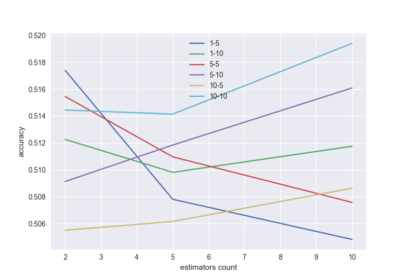
Gradient boosting with possible search over the length of the series and the window (in a good model with an increase in the number of trees, the accuracy should increase, so you need to choose the appropriate length of the series and the window):

 # gradient boosting import numpy as np import matplotlib.pyplot as plt from sklearn.model_selection import KFold, cross_val_score from sklearn.ensemble import GradientBoostingClassifier from PatternsCollector import get_patterns_for_window_and_num, get_x_y_for_patterns import seaborn nums = [2,5,10] i = 0 wrange = [1,5,10] lrange = [5,10] values = list() legends = list() for wnd in wrange: for l in lrange: scores = [] patterns = get_patterns_for_window_and_num(wnd, l) X, y = get_x_y_for_patterns(patterns, 'buy') for n in nums: i = i+1 kf = KFold(n_splits=5, shuffle=True, random_state=100) model = GradientBoostingClassifier(n_estimators=n, random_state=100) ms = cross_val_score(model, X, y, cv=kf, scoring='roc_auc') scores.append(np.mean(ms)) print 'Calculated {0}-{1}, num={2}, {3:.3f}%'.format(wnd, l, n, 100 * i/float((len(nums)*len(wrange)*len(lrange)))) values.append(scores) legends.append('{0}-{1}'.format(wnd, l)) plt.xlabel('estimators count') plt.ylabel('accuracy') for v in values: plt.plot(nums, v) plt.legend(legends) plt.show() 

Similarly, linear regression with parameter settings:

 # logistic regression from sklearn.linear_model import LogisticRegression from sklearn.preprocessing import StandardScaler from PatternsCollector import get_patterns_for_window_and_num, get_x_y_for_patterns from sklearn.model_selection import KFold, cross_val_score import numpy as np import matplotlib.pyplot as plt import seaborn cr = [10.0 ** i for i in range(-3, 1)] i = 0 wrange = [1,5,10] lrange = [5, 10] values = list() legends = list() for wnd in wrange: for l in lrange: scores = [] patterns = get_patterns_for_window_and_num(wnd, l) X, y = get_x_y_for_patterns(patterns, 'buy') sc = StandardScaler() X_sc = sc.fit_transform(X) for c in cr: i = i+1 kf = KFold(n_splits=5, shuffle=True, random_state=100) model = LogisticRegression(C=c, random_state=100) ms = cross_val_score(model, X_sc, y, cv=kf, scoring='roc_auc') scores.append(np.mean(ms)) print 'Calculated {0}-{1}, C={2}, {3:.3f}%'.format(wnd, l, c, 100 * i/float((len(cr)*len(wrange)*len(lrange)))) values.append(scores) legends.append('{0}-{1}'.format(wnd, l)) plt.xlabel('C value') plt.ylabel('accuracy') for v in values: plt.plot(cr, v) plt.legend(legends) plt.show() 

As I said, the conditions are incomplete. Therefore, we obtain an accuracy of only 0.52. But if you complement them, then accuracy will be better. You can try other algorithms - neural networks, random forest and many others. One should not forget about the problem of retraining - for example, with a large number of trees in a gradient boosting.

Check for errors in the code: if instead of real data in the database we take sin () from them, then for both classifiers AUC_ROC for cross-qualification will be 0.96.

Trading robot

In conclusion, I offer you the code of a trading robot that can place bids both on a demo account and on a real one. The most important thing is that when closing deals, he builds a histogram of profits on the deal, based on information received from the broker. That is, you can actually check how your trading strategy works.

 import datetime from datetime import datetime from os import path import matplotlib.pyplot as plt import oandapyV20 import oandapyV20.endpoints.orders as orders import oandapyV20.endpoints.positions as positions from oandapyV20.contrib.requests import MarketOrderRequest from oandapyV20.contrib.requests import TakeProfitDetails, StopLossDetails from oandapyV20.endpoints.accounts import AccountDetails from oandapyV20.endpoints.pricing import PricingInfo from Conf.Config import Config import seaborn config = Config() oanda = oandapyV20.API(environment=config.env, access_token = config.token) pReq = PricingInfo(config.account_id, 'instruments='+config.insName) asks = list() bids = list() long_time = datetime.now() short_time = datetime.now() if config.write_back_log: f_back_log = open(path.relpath(config.back_log_path + '/' + config.insName + '_' + datetime.datetime.now().strftime("%Y%m%d-%H%M%S"))+'.log', 'a'); time = 0 times = list() last_ask = 0 last_bid = 0 if config.write_back_log: print 'Backlog file name:', f_back_log.name f_back_log.write('DateTime,Instrument,ASK,BID,Price change,Status, Spread, Result \n') def process_data(ask, bid, status): global last_result global last_ask global last_bid global long_time global short_time if status != 'tradeable': print config.insName, 'is halted.' return asks.append(ask) bids.append(bid) times.append(time) # --- begin strategy here --- # --- end strategy here --- if len(asks) > config.maxLength: asks.pop(0) if len(bids) > config.maxLength: bids.pop(0) if len(times) > config.maxLength: times.pop(0) if config.write_back_log: f_back_log.write('%s,%s,%s,%s,%s,%s,%s \n' % (datetime.datetime.now(), config.insName, pReq.response.get('prices')[0].get('asks')[1].get('price'), pReq.response.get('prices')[0].get('bids')[1].get('price'), pChange, ask-bid, result)) def do_long(ask): if config.take_profit_value!=0 or config.stop_loss_value!=0: order = MarketOrderRequest(instrument=config.insName, units=config.lot_size, takeProfitOnFill=TakeProfitDetails(price=ask+config.take_profit_value).data, stopLossOnFill=StopLossDetails(price=ask-config.stop_loss_value).data) else: order = MarketOrderRequest(instrument=config.insName, units=config.lot_size) r = orders.OrderCreate(config.account_id, data=order.data) resp = oanda.request(r) print resp price = resp.get('orderFillTransaction').get('price') print time, 's: BUY price =', price return float(price) def do_short(bid): if config.take_profit_value!=0 or config.stop_loss_value!=0: order = MarketOrderRequest(instrument=config.insName, units=-config.lot_size, takeProfitOnFill=TakeProfitDetails(price=bid+config.take_profit_value).data, stopLossOnFill=StopLossDetails(price=bid-config.stop_loss_value).data) else: order = MarketOrderRequest(instrument=config.insName, units=-config.lot_size) r = orders.OrderCreate(config.account_id, data=order.data) resp = oanda.request(r) print resp price = resp.get('orderFillTransaction').get('price') print time, 's: SELL price =', price return float(price) def do_close_long(): try: r = positions.PositionClose(config.account_id, 'EUR_USD', {"longUnits": "ALL"}) resp = oanda.request(r) print resp pl = resp.get('longOrderFillTransaction').get('pl') real_profits.append(float(pl)) print time, 's: Closed. Profit = ', pl, ' price = ', resp.get('longOrderFillTransaction').get('price') except: print 'No long units to close' def do_close_short(): try: r = positions.PositionClose(config.account_id, 'EUR_USD', {"shortUnits": "ALL"}) resp = oanda.request(r) print resp pl = resp.get('shortOrderFillTransaction').get('tradesClosed')[0].get('realizedPL') real_profits.append(float(pl)) print time, 's: Closed. Profit = ', pl, ' price = ', resp.get('shortOrderFillTransaction').get('price') except: print 'No short units to close' def get_bal(): r = AccountDetails(config.account_id) return oanda.request(r).get('account').get('balance') plt.ion() plt.grid(True) do_close_long() do_close_short() real_profits = list() while True: try: oanda.request(pReq) ask = float(pReq.response.get('prices')[0].get('asks')[0].get('price')) bid = float(pReq.response.get('prices')[0].get('bids')[0].get('price')) status = pReq.response.get('prices')[0].get('status') process_data(ask, bid, status) plt.clf() plt.subplot(1,2,1) plt.plot(times, asks, color='red', label='ASK') plt.plot(times, bids, color='blue', label='BID') if last_ask!=0: plt.axhline(last_ask, linestyle=':', color='red', label='curr ASK') if last_bid!=0: plt.axhline(last_bid, linestyle=':', color='blue', label='curr BID') plt.xlabel('Time, s') plt.ylabel('Price change') plt.legend(loc='upper left') plt.subplot(1, 2, 2) plt.hist(real_profits, label='Profits') plt.legend(loc='upper left') plt.xlabel('Profits') plt.ylabel('Counts') plt.tight_layout() except Exception as e: print e plt.pause(config.period) time = time + config.period 

Full source code here .

I hope that I saved time for those who are interested in algotrading. After all, now to check your ideas you only need to change the code a bit, run the robot and get statistics on your transactions from the broker. And you can analyze almost any stock data.

Special thanks I want to say to the authors of the course Yandex for machine learning on Coursera. And also Andrew Ng for the wonderful lectures on the same resource.

UPDATE:
But what happens on the gradient boosting on the glued SI futures from the final over the last year (if the criterion for choosing a pattern is a 1% price jump to the right direction):

And this is a good result. Expectation plus.
And just then Alpha Direct has released a new server API :)