Harmonic Linearization with Python Tools

Why do you need it

The harmonic linearization method is widely used to analyze nonlinear systems [1]. This method is used to determine the conditions for the occurrence of self-oscillations in systems of the second and higher order. With harmonic linearization, the following two conditions must be met. A closed linear system should consist of two parts: linear and nonlinear. The linear part should have good filtering properties for higher harmonics [2]. Automatic control and regulation systems contain actuators containing non-linear elements, therefore their analysis is a very topical issue.

Main algorithm

Let the harmonic signal be input to the nonlinear element

where

By converting the output signal to a Fourier series for the first harmonic only. We get:

Taking into account (1), (2), the general equation of a nonlinear element can be represented as [3]:

where ─ real "a" is the imaginary component of the harmonic linearization coefficient obtained from the condition of the subsequent filtering of higher harmonics; ─ circular frequency; - differentiation operator.
')

Formulation of the problem

We will compare the two nonlinear elements shown in Figure 1.2, in order to determine the amplitude stability.

Fig.1 Nonlinearity type "saturation"

Using (1), while only for the real part, we get:

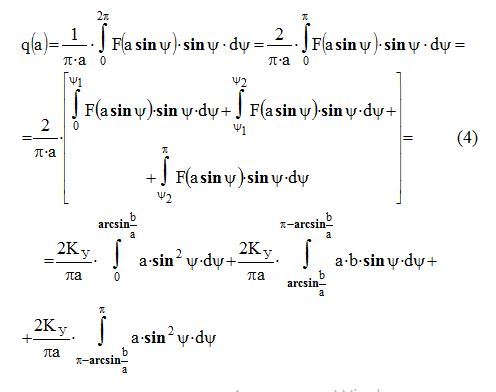
Fig.2 Non-linearity type "break"

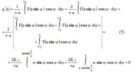
Similarly, using (1), while only for the real part, we get:

Implementation (4), (5) in Python

#!/usr/bin/python # -*- coding: utf-8 -*- import matplotlib.pyplot as plt #     import matplotlib as mpl #    mpl.rcParams['font.family'] = 'fantasy'#  mpl.rcParams['font.fantasy'] = 'Comic Sans MS, Aria'#  import scipy.integrate as spint #     import math #     import numpy as np#      q=[]#    - p=[]#   - c=[]#      k=1#     for m in np.arange(1.0,4,0.1): #     def f(x): #       return k*(math.sin(x))**2 a = 0#    b =math.asin(1/m)#    z=spint.quad(f,a,b)[0]#   a =math.pi-math.asin(1/m)#   b =math.pi#   z1=spint.quad(f,a,b)[0]#  q.append(round(z+z1,3))#    -  def f1(x):#       return (k/m)*(math.sin(x)) a =math.asin(1/m)#   b =math.pi-math.asin(1/m)#   z2=spint.quad(f1,a,b)[0] #  p.append(round(z+z1+z2,3))#   -  x=np.arange(1.0,4,0.1)#        x2=np.arange(0.0,1.1,0.1)#        for i in np.arange(0.0,1.1,0.1):#      c.append(p[0]) plt.title('  ', size=14)#   plt.xlabel('  ', size=14)#     plt.ylabel('  ', size=14)#     plt.plot(x, q, color='r', linewidth=2, label='-- ')#     plt.plot(x, p, color='b',linewidth=2, label=' ')#    plt.plot(x2, c, color='g', linewidth=2, label=' ')#    plt.legend(loc='best')#    plt.grid(True)#  plt.show()#

Result (yes in jpeg, but this is a graph!)

By the way, integration using import scipy.integrate as spint is carried out stably and without errors.

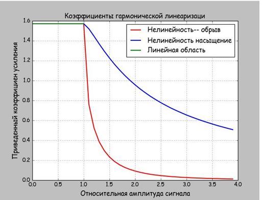
From the graph, it is clear that the nonlinear element shown in Fig. 2, provided that the harmonics are filtered, will provide greater amplitude stability than that shown in Fig. 1. A more detailed analysis will show a smaller percentage of harmonics, but this is the topic of another article.

You, of course, ask, "But what about the other non-linearities, maybe they are even better?". I did this for a low-frequency (up to 5 kHz) special purpose amplifier with typical characteristics shown in Figure 1.2. By the way, the characteristics of Figure 2 are not in any reference.

Option code reduction program

You can use symbolic calculations, for example, like this:

 from sympy import * import matplotlib.pyplot as plt import numpy as np x=Symbol('x') m=Symbol('m') z=integrate(sin(x)**2, (x,0,asinh(m)))+integrate(sin(x)**2, (x,pi-asinh(m),pi)) #    -  z1=integrate(sin(x)**2, (x,0,asinh(m)))+integrate(m*sin(x), (x,asinh(m),pi-asinh(m)) )+integrate(sin(x)**2, (x,pi-asinh(m),pi))#     print(z) print(z1)

We get: -sin (asinh (m)) * cos (asinh (m)) + asinh (m)
2 * m * cos (asinh (m)) - sin (asinh (m)) * cos (asinh (m)) + asinh (m)

Software simplification (simplify (z)) does nothing, so we use the relations:

, we get:

Enter the ratio of the amplitude to the threshold of limitation and finally get:

Relation (6) the solution of equation (5), system (7) the solution of equation (4).

findings

The article describes the method of comparative analysis of nonlinear elements by the method of harmonic linearization.