Practical application of Fourier transform for signal processing
Introduction
Books and publications on digital signal processing are written by authors who often do not guess and do not understand the tasks facing the developers. This is especially true of real-time systems. These authors devote themselves to the modest role of a god who exists outside of time and space, which causes some perplexity in readers of such literature. This publication is intended to dispel the misunderstandings that arise among the majority of developers and help them overcome the “threshold of entry”; for these purposes, the text consciously uses analogies and terminology of the programming sphere.
This opus does not claim completeness and coherence.
Added after reading the comments.
Publications about how to do FFT nemeryannom, but about how to do FFT, transform the spectrum, and collect the signal again, and even in real time, is clearly not enough. The author is trying to fill this gap.
')
Part one, overview
There are two main ways to build discrete linear dynamic systems. In the literature, such systems are called digital filters, which are divided into two main types: filters with finite impulse response (FIR) and filters with infinite impulse response (IIR).
The algorithm essence of the FIR filter is the discrete calculation of the convolution integral:

Where x (t) is the input signal
y (t) - output signal
h (t) is the filter impulse response or filter response to the delta function. The impulse response is the inverse Fourier transform of the complex frequency response of the filter K (f).
To form a clear picture with the reader, we give an example of a discrete calculation of the convolution integral in C in real time.
Calling this function at certain time intervals T and passing the input signal as an argument to it, we will get an output signal corresponding to the filter response with an impulse response of the form:
h (t) = 1 at 0 <t <4T,
h (t) = 0 in other cases.
The filter with such an impulse characteristic is better known to all those gathered under the name “moving average filter”, and, accordingly, it is implemented much easier. In this case, this impulse response is used as an example.
A lot of literature is devoted to the synthesis of pulse characteristics of FIR filters; there are also ready-made software products for obtaining filters with specified properties. The author prefers the buggy Filter Design tool from the Matlab package, but this is a matter of taste.
Using a filter with a finite impulse response, it is possible to soar a little over the usual reality, since, in nature, there are no dynamic systems that have a finite impulse response. The FIR filter is an attempt to enter the time-frequency domain from the other end, not as nature walks, therefore the frequency characteristics of these filters often have unexpected properties.
Much closer to nature are filters with infinite impulse response. The algorithmic essence of filters with infinite impulse response is reduced to a recurrent (not to be confused with a recursive!) Solution of a differential equation describing a filter. That is, each subsequent value of the output signal of the filter is calculated based on the previous value. That is how the processes in the real world proceed. The stone, falling from a skyscraper every second, increases its speed by 9.8m / s Speed = Speed + 9.8, and the distance traveled every second increases Distance = Distance + Speed. Who can say that this is not a recurrent algorithm, let the first one throw a stone at me. Only in our Matrix, the time interval for calling the function returning the position of a stone is much less than the cost of dividing the means of measurement available to us.
Separately, I would like to define the concept of "filter order". This is the number of variables that undergo recurrent operations. In the above example, the function that returns the speed of the stone is of the first order, the function that returns the distance traveled is of the second order.
For the final clarification of the reader, we will give an example in the C language of the simplest low-pass filter, commonly known as the filter “filter of exponential smoothing”
Calling this function with the frequency F and passing it the input signal as an argument, we will get the output signal corresponding to the response of the low-pass filter of the first order with the cutoff frequency:
The given example of source code is completely indigestible from the point of view of understanding the essence of the algorithm. From the point of view of the recurrent essence (see the “stone fall”) of the algorithm, more correctly y = y + ((xy) >> alfa); but in this case there is a loss of alfa of significant digits. The recurrent expression of the filter, from the sample code, is constructed in such a way as to avoid the loss of significant digits. It is the finite accuracy of calculations that can spoil the beauty of a digital filter with infinite impulse response. This is especially noticeable on high-order filters characterized by high Q-factors. In real dynamic systems, this problem does not arise, our Matrix performs calculations with incredible accuracy for us.
A lot of literature is devoted to the synthesis of such filters, there are also ready-made software products (see above).
Part two. Fourier filter
From university courses (for your humble servant, this was the OTETS course), many gathered remember two main approaches to the analysis of linear dynamic systems: analysis in the time domain and analysis in the frequency domain. The analysis in the time domain is the solution of differential equations, convolution and Duhamel integrals. These analysis methods are discretely embodied in IIR and KIH digital filters.
But there is a frequency approach to the analysis of linear dynamic systems. Sometimes it is called operator. The operators used are Fourier transform, Laplace, etc. Further we will talk only about the Fourier transform.
This method of analysis is not widely used in the construction of digital filters. The author could not find any sane practical recommendations for building such filters in Russian. The only brief mention of such a filter in the practical literature [Rabiner L., Gould B., Theory and application of digital signal processing 1978], but in this book, the consideration of such a filter is very superficial. In this book, this filter scheme is called: “convolution in real time by the FFT method”, which, in my humble opinion, does not reflect the essence, the name should be short, otherwise there will be no time to rest.
The reaction of a linear dynamic system is the inverse Fourier transform of the product of the Fourier image of the input signal x (t) by the complex transfer coefficient K (f):
In practical terms, this analytical expression suggests the following procedure: take the Fourier transform from the input signal, multiply the result by the complex transfer coefficient, perform the inverse Fourier transform, which results in the output signal. In real discrete time, this procedure cannot be performed. How to take the integral in time from minus to plus infinity? It can be taken only being out of time ...
In the discrete world, there is a tool for performing the Fourier transform — the Fast Fourier Transform Algorithm (FFT). That is what we will use when implementing our Fourier filter. The argument of the FFT function is an array of time samples of 2 ^ n elements, the result of two arrays of length 2 ^ n elements corresponding to the real and imaginary parts of the Fourier transform. A discrete feature of the FFT algorithm is that the input signal is considered periodic with an interval of 2 ^ n. This imposes some restrictions on the Fourier filter algorithm. If you take a sequence of samples of the input signal, perform an FFT from them, multiply the result of the FFT by the complex filter transfer coefficient and perform the inverse transformation ... nothing happens! The output signal will have huge non-linear distortions in the vicinity of the sample junctions.
To solve this problem, you need to apply two techniques:

Such functions are widely used in the technique of digital signal processing, and it is customary to call them windows. According to the author’s humble opinion, the best, from a practical point of view, is the window of the Khan name:
The figure shows graphs illustrating the properties of a Han window with a length of 2 ^ n = 256. Window instances are built with a half overlap of k = 128. As you can see all the above properties are available.
At the request of workers, the following figure shows the Fourier filter calculation scheme, with a sample length of 2 ^ n = 8, number of samples 3. In such figures it is very difficult to display the calculation process, it is especially hard to show its cyclicality, therefore we limited ourselves to the number of samples .

The input signal is divided into blocks of length 2 ^ n = 8 with overlap of 50%, FFT is taken from each block, the FFT results undergo the required transformation, the inverse FFT is taken, the result of the inverse FFT is multiplied scalarly by the window, after multiplication, the blocks are added to overlap.
When performing spectrum transformations, you should not forget about the main property of the FFT array of real signals, the first half of the FFT array is complexly conjugated with the second half, that is, Re [i] = Re [(1 << n) -i]); Im [i] = - Im [(1 << n) -i]) ;. If these requirements do not fulfill the output signal simply "does not meet."
Now we know everything that is needed to write a Fourier filter algorithm. We describe the algorithm in C.
Calling the FureFilter () function with the FSempl frequency and passing it the input signal as an argument, we get the output signal. In this example, the input signal is processed as follows: the signal is passed through a band-pass filter with cut-off frequencies FsrLow, FsrHi, all spectral components above and below the frequencies are suppressed, the signal spectrum is shifted (for sound signals this is perceived as the Buratino-Karabas effect), the amplitude spectrum of the signal it is smoothed by a low-pass filter (for sound, this is the effect of a booming room). These actions with a signal are performed as an example in order to show technical methods of signal processing in the frequency domain, such as: observance of complex conjugacy of coefficients, reconstruction of the complex amplitude spectrum, without using trigonometric functions, etc.
Conclusion
It is worth noting that, most likely, this Fourier filter function, in practice, will be disabled. By calling this function, even with a low frequency of 8000 Hz, it will not have time to be executed by the time of the next call, there is not enough speed. This program code of the Fourier filter is given as a description of the algorithm, without being tied to specific hardware resources, and has purely educational purposes (see Introduction).
In practical implementation, it is necessary to parallelize the execution of the function of filling-emptying the buffer BufInOut [] (it is better to immediately use the RAP, etc.) and the function of processing the buffer ObrBuf (), but this is a completely different story.
Books and publications on digital signal processing are written by authors who often do not guess and do not understand the tasks facing the developers. This is especially true of real-time systems. These authors devote themselves to the modest role of a god who exists outside of time and space, which causes some perplexity in readers of such literature. This publication is intended to dispel the misunderstandings that arise among the majority of developers and help them overcome the “threshold of entry”; for these purposes, the text consciously uses analogies and terminology of the programming sphere.
This opus does not claim completeness and coherence.
Added after reading the comments.
Publications about how to do FFT nemeryannom, but about how to do FFT, transform the spectrum, and collect the signal again, and even in real time, is clearly not enough. The author is trying to fill this gap.
')
Part one, overview
There are two main ways to build discrete linear dynamic systems. In the literature, such systems are called digital filters, which are divided into two main types: filters with finite impulse response (FIR) and filters with infinite impulse response (IIR).
The algorithm essence of the FIR filter is the discrete calculation of the convolution integral:
Where x (t) is the input signal
y (t) - output signal
h (t) is the filter impulse response or filter response to the delta function. The impulse response is the inverse Fourier transform of the complex frequency response of the filter K (f).
To form a clear picture with the reader, we give an example of a discrete calculation of the convolution integral in C in real time.
#define L (4) // int FIR(int a) { static int i=0; // static int reg[L]; // static const int h[L]={1,1,1,1};// int b=0;// reg[i]=a; // for(int j=0;j<L;j++)// { b=b+h[j]*reg[i]; i=(i-1)&(L-1); } i=(i+1)&(L-1);// return b; } Calling this function at certain time intervals T and passing the input signal as an argument to it, we will get an output signal corresponding to the filter response with an impulse response of the form:
h (t) = 1 at 0 <t <4T,
h (t) = 0 in other cases.
The filter with such an impulse characteristic is better known to all those gathered under the name “moving average filter”, and, accordingly, it is implemented much easier. In this case, this impulse response is used as an example.
A lot of literature is devoted to the synthesis of pulse characteristics of FIR filters; there are also ready-made software products for obtaining filters with specified properties. The author prefers the buggy Filter Design tool from the Matlab package, but this is a matter of taste.
Using a filter with a finite impulse response, it is possible to soar a little over the usual reality, since, in nature, there are no dynamic systems that have a finite impulse response. The FIR filter is an attempt to enter the time-frequency domain from the other end, not as nature walks, therefore the frequency characteristics of these filters often have unexpected properties.
Much closer to nature are filters with infinite impulse response. The algorithmic essence of filters with infinite impulse response is reduced to a recurrent (not to be confused with a recursive!) Solution of a differential equation describing a filter. That is, each subsequent value of the output signal of the filter is calculated based on the previous value. That is how the processes in the real world proceed. The stone, falling from a skyscraper every second, increases its speed by 9.8m / s Speed = Speed + 9.8, and the distance traveled every second increases Distance = Distance + Speed. Who can say that this is not a recurrent algorithm, let the first one throw a stone at me. Only in our Matrix, the time interval for calling the function returning the position of a stone is much less than the cost of dividing the means of measurement available to us.
Separately, I would like to define the concept of "filter order". This is the number of variables that undergo recurrent operations. In the above example, the function that returns the speed of the stone is of the first order, the function that returns the distance traveled is of the second order.
For the final clarification of the reader, we will give an example in the C language of the simplest low-pass filter, commonly known as the filter “filter of exponential smoothing”
#define alfa (2) // int filter(int a) { static int out_alfa=0; out_alfa=out_alfa - (out_alfa >>alfa) + a; return (out_alfa >> alfa); } Calling this function with the frequency F and passing it the input signal as an argument, we will get the output signal corresponding to the response of the low-pass filter of the first order with the cutoff frequency:
The given example of source code is completely indigestible from the point of view of understanding the essence of the algorithm. From the point of view of the recurrent essence (see the “stone fall”) of the algorithm, more correctly y = y + ((xy) >> alfa); but in this case there is a loss of alfa of significant digits. The recurrent expression of the filter, from the sample code, is constructed in such a way as to avoid the loss of significant digits. It is the finite accuracy of calculations that can spoil the beauty of a digital filter with infinite impulse response. This is especially noticeable on high-order filters characterized by high Q-factors. In real dynamic systems, this problem does not arise, our Matrix performs calculations with incredible accuracy for us.
A lot of literature is devoted to the synthesis of such filters, there are also ready-made software products (see above).
Part two. Fourier filter
From university courses (for your humble servant, this was the OTETS course), many gathered remember two main approaches to the analysis of linear dynamic systems: analysis in the time domain and analysis in the frequency domain. The analysis in the time domain is the solution of differential equations, convolution and Duhamel integrals. These analysis methods are discretely embodied in IIR and KIH digital filters.
But there is a frequency approach to the analysis of linear dynamic systems. Sometimes it is called operator. The operators used are Fourier transform, Laplace, etc. Further we will talk only about the Fourier transform.
This method of analysis is not widely used in the construction of digital filters. The author could not find any sane practical recommendations for building such filters in Russian. The only brief mention of such a filter in the practical literature [Rabiner L., Gould B., Theory and application of digital signal processing 1978], but in this book, the consideration of such a filter is very superficial. In this book, this filter scheme is called: “convolution in real time by the FFT method”, which, in my humble opinion, does not reflect the essence, the name should be short, otherwise there will be no time to rest.
The reaction of a linear dynamic system is the inverse Fourier transform of the product of the Fourier image of the input signal x (t) by the complex transfer coefficient K (f):
In practical terms, this analytical expression suggests the following procedure: take the Fourier transform from the input signal, multiply the result by the complex transfer coefficient, perform the inverse Fourier transform, which results in the output signal. In real discrete time, this procedure cannot be performed. How to take the integral in time from minus to plus infinity? It can be taken only being out of time ...
In the discrete world, there is a tool for performing the Fourier transform — the Fast Fourier Transform Algorithm (FFT). That is what we will use when implementing our Fourier filter. The argument of the FFT function is an array of time samples of 2 ^ n elements, the result of two arrays of length 2 ^ n elements corresponding to the real and imaginary parts of the Fourier transform. A discrete feature of the FFT algorithm is that the input signal is considered periodic with an interval of 2 ^ n. This imposes some restrictions on the Fourier filter algorithm. If you take a sequence of samples of the input signal, perform an FFT from them, multiply the result of the FFT by the complex filter transfer coefficient and perform the inverse transformation ... nothing happens! The output signal will have huge non-linear distortions in the vicinity of the sample junctions.
To solve this problem, you need to apply two techniques:
- 1. Samples must be processed by overlapping Fourier transform. That is, each subsequent sample should contain a part of the previous one. In the ideal case, the samples should overlap by (2 ^ n-1) samples, but this requires a huge computational cost. In practice, more than three quarters (2 ^ n-2 ^ (n-2)), half (2 ^ (n-1)) and even a quarter overlap (2 ^ (n-2)) are sufficient.
- 2. The results of the inverse Fourier transform, to obtain the output signal, it is necessary, before imposing on each other, multiplied by the weight function (an array of weights). The weight function must satisfy the following conditions:
- 2.1 Equal to zero everywhere except for the interval 2 ^ n.
- 2.2 At the edges of the interval tends to zero.
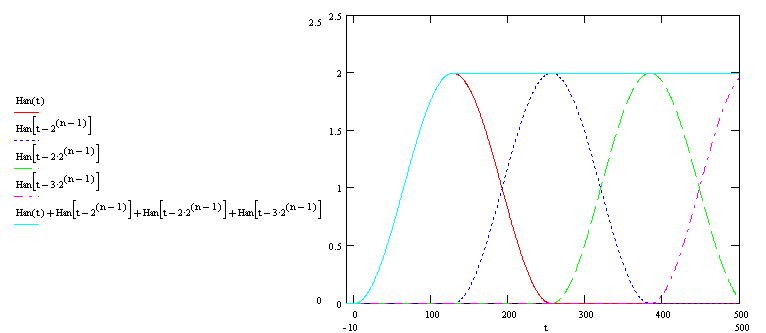
- 2.3 And, most importantly, the sum of the weight functions Fv (t) shifted by the overlap interval k should be constant:
Such functions are widely used in the technique of digital signal processing, and it is customary to call them windows. According to the author’s humble opinion, the best, from a practical point of view, is the window of the Khan name:
The figure shows graphs illustrating the properties of a Han window with a length of 2 ^ n = 256. Window instances are built with a half overlap of k = 128. As you can see all the above properties are available.
At the request of workers, the following figure shows the Fourier filter calculation scheme, with a sample length of 2 ^ n = 8, number of samples 3. In such figures it is very difficult to display the calculation process, it is especially hard to show its cyclicality, therefore we limited ourselves to the number of samples .
The input signal is divided into blocks of length 2 ^ n = 8 with overlap of 50%, FFT is taken from each block, the FFT results undergo the required transformation, the inverse FFT is taken, the result of the inverse FFT is multiplied scalarly by the window, after multiplication, the blocks are added to overlap.
When performing spectrum transformations, you should not forget about the main property of the FFT array of real signals, the first half of the FFT array is complexly conjugated with the second half, that is, Re [i] = Re [(1 << n) -i]); Im [i] = - Im [(1 << n) -i]) ;. If these requirements do not fulfill the output signal simply "does not meet."
Now we know everything that is needed to write a Fourier filter algorithm. We describe the algorithm in C.
#include <math.h> #define FSempl (8000)// #define BufL (64) // #define Perk (2) // 2-1/2, 4-3/4 // , #define FsrLow (300)// #define FsrHi (3100)// #define FsrLowN ((BufL*FsrLow+(FSempl/2))/FSempl)// #define FsrHiN ((BufL*FsrHi +(FSempl/2))/FSempl)// // #define SdvigSp (0)// +() -() 0( ) // , #define FilterSpekrtaT_EN (1)// 1/0 #define FiltSpektrFsr (0.100025f) // volatile unsigned short ShBuf;// signed short BufIn[BufL*2];// signed short BufOut[BufL*2];// signed short BufInOut[BufL];// float FurRe[BufL];// float FurIm[BufL];// #if (FilterSpekrtaT_EN!=0) float FStektr[BufL/2];// #endif // #if BufL==64 const float SinCosF[]= { 0.000000000 , 0.098017140 , 0.195090322 , 0.290284677 , 0.382683432 , 0.471396737 , 0.555570233 , 0.634393284 , 0.707106781 , 0.773010453 , 0.831469612 , 0.881921264 , 0.923879533 , 0.956940336 , 0.980785280 , 0.995184727 , 1.000000000 , 0.995184727 , 0.980785280 , 0.956940336 , 0.923879533 , 0.881921264 , 0.831469612 , 0.773010453 , 0.707106781 , 0.634393284 , 0.555570233 , 0.471396737 , 0.382683432 , 0.290284677 , 0.195090322 , 0.098017140 , 0.000000000 , -0.098017140, -0.195090322, -0.290284677, -0.382683432, -0.471396737, -0.555570233, -0.634393284, -0.707106781, -0.773010453, -0.831469612, -0.881921264, -0.923879533, -0.956940336, -0.980785280, -0.995184727, -1.000000000, -0.995184727, -0.980785280, -0.956940336, -0.923879533, -0.881921264, -0.831469612, -0.773010453, -0.707106781, -0.634393284, -0.555570233, -0.471396737, -0.382683432, -0.290284677, -0.195090322, -0.098017140, 0.000000000 , 0.098017140 , 0.195090322 , 0.290284677 , 0.382683432 , 0.471396737 , 0.555570233 , 0.634393284 , 0.707106781 , 0.773010453 , 0.831469612 , 0.881921264 , 0.923879533 , 0.956940336 , 0.980785280 , 0.995184727 }; #endif // #if BufL==64 const unsigned short sortFFT[]= { 0x0000,0x0020,0x0010,0x0030,0x0008,0x0028,0x0018,0x0038, 0x0004,0x0024,0x0014,0x0034,0x000C,0x002C,0x001C,0x003C, 0x0002,0x0022,0x0012,0x0032,0x000A,0x002A,0x001A,0x003A, 0x0006,0x0026,0x0016,0x0036,0x000E,0x002E,0x001E,0x003E, 0x0001,0x0021,0x0011,0x0031,0x0009,0x0029,0x0019,0x0039, 0x0005,0x0025,0x0015,0x0035,0x000D,0x002D,0x001D,0x003D, 0x0003,0x0023,0x0013,0x0033,0x000B,0x002B,0x001B,0x003B, 0x0007,0x0027,0x0017,0x0037,0x000F,0x002F,0x001F,0x003F }; #endif // #if BufL==64 const float WinHanF[]= { 0.0 , 0.002407637 , 0.00960736 , 0.021529832 , 0.038060234 , 0.059039368 , 0.084265194 , 0.113494773 , 0.146446609 , 0.182803358 , 0.222214883 , 0.264301632 , 0.308658284 , 0.354857661 , 0.402454839 , 0.45099143 , 0.5 , 0.54900857 , 0.597545161 , 0.645142339 , 0.691341716 , 0.735698368 , 0.777785117 , 0.817196642 , 0.853553391 , 0.886505227 , 0.915734806 , 0.940960632 , 0.961939766 , 0.978470168 , 0.99039264 , 0.997592363 , 1.0 , 0.997592363 , 0.99039264 , 0.978470168 , 0.961939766 , 0.940960632 , 0.915734806 , 0.886505227 , 0.853553391 , 0.817196642 , 0.777785117 , 0.735698368 , 0.691341716 , 0.645142339 , 0.597545161 , 0.54900857 , 0.5 , 0.45099143 , 0.402454839 , 0.354857661 , 0.308658284 , 0.264301632 , 0.222214883 , 0.182803358 , 0.146446609 , 0.113494773 , 0.084265194 , 0.059039368 , 0.038060234 , 0.021529832 , 0.00960736 , 0.002407637 }; #endif //@@@@@@@@@@@@@@@@@@@@@@@@@@@@@@@@@@@@@@@@@@@@@@@@@@@@@@@@@@@@@@@@@@@@@@@@@@@@@ // // // ReFT ImFT // . void FFTnoInv(float* ReFT,float* ImFT) { // for(int i=0;i<BufL;i++) { int j=sortFFT[i];// if(i<j)// { // float swp=ReFT[i]; ReFT[i]=ReFT[j]; ReFT[j]=swp; // //swp=ImFT[i]; //ImFT[i]=ImFT[j]; //ImFT[j]=swp; } } // long darg=BufL; // for(long LP2=1;LP2!=BufL;LP2=LP2<<1)// { darg=darg>>1; long arg=0; // , for(int j=0;j<LP2;j++) // { float c=(SinCosF[arg+(BufL/4)]);// float s=(SinCosF[arg]);// arg=(arg-darg)&(BufL-1);// for(int i=j;i<BufL;i=(i+LP2+LP2)) // { //!!! float wr=(c*ReFT[i+LP2])-(s*ImFT[i+LP2]); float wi=(s*ReFT[i+LP2])+(c*ImFT[i+LP2]); ReFT[i+LP2]=ReFT[i]-wr; ImFT[i+LP2]=ImFT[i]-wi; ReFT[ i ]=ReFT[i]+wr; ImFT[ i ]=ImFT[i]+wi; } } } // return; } //@@@@@@@@@@@@@@@@@@@@@@@@@@@@@@@@@@@@@@@@@@@@@@@@@@@@@@@@@@@@@@@@@@@@@@@@@@@@@ // // // ReFT ImFT // . // 0 void FFTInv(float* ReFT,float* ImFT) { // for(int i=0;i<BufL;i++) { int j=sortFFT[i];// if(i<j)// { // float swp=ReFT[i]; ReFT[i]=ReFT[j]; ReFT[j]=swp; swp=ImFT[i]; ImFT[i]=ImFT[j]; ImFT[j]=swp; } } // long darg=BufL;// for(long LP2=1;LP2!=BufL;LP2=LP2<<1)// { darg=darg>>1; long arg=0;//// , for(int j=0;j<LP2;j++)// { float c=(SinCosF[arg+(BufL/4)]);// float s=(SinCosF[arg]);// arg=arg+darg;// for(int i=j;i<BufL;i=(i+LP2+LP2))// { //!!! float wr=(c*ReFT[i+LP2])-(s*ImFT[i+LP2]); float wi=(s*ReFT[i+LP2])+(c*ImFT[i+LP2]); ReFT[i+LP2]=ReFT[i]-wr; ImFT[i+LP2]=ImFT[i]-wi; ReFT[ i ]=ReFT[i]+wr; ImFT[ i ]=ImFT[i]+wi; } } } //, for(int i=0;i<BufL;i++) { ReFT[i]=ReFT[i] * WinHanF[i] * ( (1.0F/((float)BufL)) * (2.0F/((float)Perk)) ); } // return; } //@@@@@@@@@@@@@@@@@@@@@@@@@@@@@@@@@@@@@@@@@@@@@@@@@@@@@@@@@@@@@@@@@@@@@@@@@@@@@ // void ObrBuf(void) { // for(int i=0;i<(BufL);i++) { FurRe[i]=((float)BufInOut[i]); FurIm[i]=0.0F; } // FFTnoInv(FurRe,FurIm); // #if SdvigSp>0 // , - for(int i=1;i<(BufL/2);i++) { if(i>=(BufL/2-SdvigSp)) { FurRe[i]=FurIm[i]=0; FurRe[BufL-i]=FurIm[BufL-i]=0; continue; } FurRe[i]=FurRe[i+SdvigSp]; FurIm[i]=FurIm[i+SdvigSp]; FurRe[BufL-i]=FurRe[i]; FurIm[BufL-i]=-FurIm[i]; } #endif #if SdvigSp<0 // , for(int i=(BufL/2-1);i>0;i--) { if(i<=(-SdvigSp)) { FurRe[i]=FurIm[i]=0; FurRe[BufL-i]=FurIm[BufL-i]=0; continue; } FurRe[i]=FurRe[i-(-SdvigSp)]; FurIm[i]=FurIm[i-(-SdvigSp)]; FurRe[BufL-i]=FurRe[i]; FurIm[BufL-i]=-FurIm[i]; } #endif // , FurRe[0]=0.0F;FurIm[0]=0.0F; // FurRe[(BufL/2)]=0.0F;FurIm[(BufL/2)]=0.0F;// float ZnStektr[BufL/2];// for(int i=1;i<(BufL/2);i++) { if( ( i < FsrLowN )// || ( i > FsrHiN )// ) { // , FurRe[i]=0.0F;FurIm[i]=0.0F;// FurRe[BufL-i]=0.0F;FurIm[BufL-i]=0.0F;// } else // { ZnStektr[i]=sqrtf(FurRe[i]*FurRe[i])+(FurIm[i]*FurIm[i]);// } } // , for(int i= FsrLowN;// i<=FsrHiN ;// i++) { #if FilterSpekrtaT_EN!=0 // , FStektr[i]=FStektr[i]+ FiltSpektrFsr*(ZnStektr[i]-FStektr[i]); #endif // FurRe[i]=FurRe[BufL-i]=(FStektr[i]*FurRe[i])/ZnStektr[i]; FurIm[i]=(FStektr[i]*FurIm[i])/ZnStektr[i]; FurIm[BufL-i]=-FurIm[i]; } // FFTInv(FurRe,FurIm); // for(int i=0;i<(BufL);i++) { BufInOut[i]=((signed short)(FurRe[i]+0.5f)); } } //@@@@@@@@@@@@@@@@@@@@@@@@@@@@@@@@@@@@@@@@@@@@@@@@@@@@@@@@@@@@@@@@@@@@@@@@@@@@@ // signed short FureFilter(signed short t1) { // BufIn[ShBuf]=t1; // signed short out=BufOut[ShBuf]; // ShBuf=(ShBuf+1)&((BufL*2)-1); // if((ShBuf&((BufL/Perk)-1))==0) { // int ShTmpOut=ShBuf; int ShTmpIn=(ShBuf-BufL)&((BufL*2)-1); for(int i=0;i<(BufL);i++) { if(i<(BufL-(BufL/Perk))) { // BufOut[ShTmpOut]=BufOut[ShTmpOut]+BufInOut[i]; } else { // BufOut[ShTmpOut]=BufInOut[i]; } // ShTmpOut=(ShTmpOut+1)&((BufL*2)-1); // BufInOut[i]=BufIn[ShTmpIn]; // ShTmpIn=(ShTmpIn+1)&((BufL*2)-1); } }// if((ShBuf&((BufL/Perk)-1))==0) // // ! if((ShBuf&((BufL/Perk)-1))==0)ObrBuf(); return out; } Calling the FureFilter () function with the FSempl frequency and passing it the input signal as an argument, we get the output signal. In this example, the input signal is processed as follows: the signal is passed through a band-pass filter with cut-off frequencies FsrLow, FsrHi, all spectral components above and below the frequencies are suppressed, the signal spectrum is shifted (for sound signals this is perceived as the Buratino-Karabas effect), the amplitude spectrum of the signal it is smoothed by a low-pass filter (for sound, this is the effect of a booming room). These actions with a signal are performed as an example in order to show technical methods of signal processing in the frequency domain, such as: observance of complex conjugacy of coefficients, reconstruction of the complex amplitude spectrum, without using trigonometric functions, etc.
Conclusion
It is worth noting that, most likely, this Fourier filter function, in practice, will be disabled. By calling this function, even with a low frequency of 8000 Hz, it will not have time to be executed by the time of the next call, there is not enough speed. This program code of the Fourier filter is given as a description of the algorithm, without being tied to specific hardware resources, and has purely educational purposes (see Introduction).
In practical implementation, it is necessary to parallelize the execution of the function of filling-emptying the buffer BufInOut [] (it is better to immediately use the RAP, etc.) and the function of processing the buffer ObrBuf (), but this is a completely different story.
Source: https://habr.com/ru/post/324152/
All Articles