Splunk. Introduction to machine data analysis - part 1. Examples of SPL queries and log visualization

In this article, we will tell and show how to load data into Splunk, how to build search queries in the system based on the integrated SPL language and how you can visualize them. This is a purely practical “How to” article based on test data , access to which is provided freely and is available for download to everyone.

After reading and repeating, you will learn:
')

• Use basic system functionality
• Upload data to Splunk
• Build basic search queries
• Visualize the results

Loading data into the system

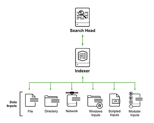
The system can be divided into 5 main sources of collecting logs (this is not a complete list):

• Files and Directories: Splunk can one-time pick up or monitor a specific file or directory with files, and independently monitors the change.
• Network events: data coming from network ports (syslog for example)
• Windows sources: Windows event logs, AD events
• Scripted Inputs: Scripted Data
• Modular Inputs: Collecting Data from Specific Platforms, Systems, and Applications

In this article, for clarity, we will use the most simple method. We simply upload the test file to Splunk from the local computer. It is clear that in the history with Enterprise use nobody does this, and the options described above are used together with the forwarder agents on the target systems, and then the infrastructure looks like this:



But in our educational example, one free Splunk Enterprise Free downloaded to the local computer will be enough for us. Installation instructions can be found in our previous article .

Now that you have downloaded the data and installed Splunk, you need to load it into it. In fact, it is quite simple ( instruction ), because the data are prepared in advance. It is important ! No need to unzip the archive.

SPL requests

Key features of the SPL language:

• 140+ search commands
• The syntax is similar to the Unix pipeline and SQL and is optimized for data with a time stamp.
• SPL allows you to search, filter, modify, enrich, combine and delete
• SPL includes machine learning and anomaly lookups.

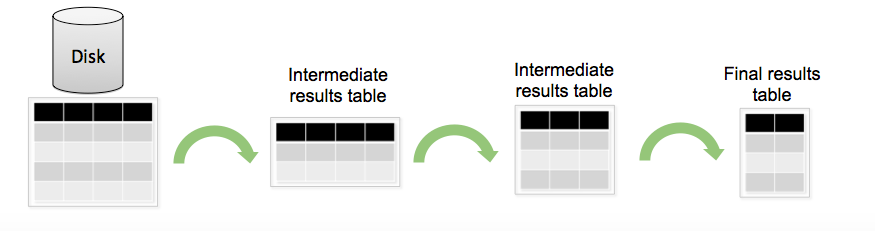
SPL structure:

Standardly, the SPL query can be divided into several stages: filtering and selecting the necessary data, then creating new fields based on existing ones, then aggregating the data and calculating statistics, and finally renaming the fields, sorting in other words, refining the output.



After you have loaded the data into the system, you can search for them (below are examples of requests, with the results of execution):

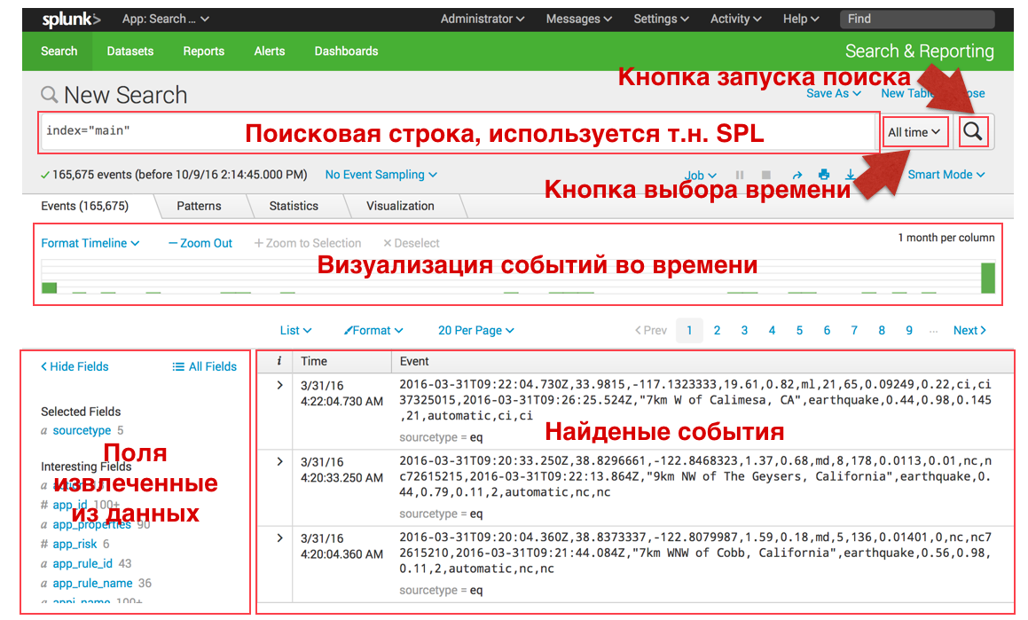
The search interface is as follows:

Search and filtering:

In Splunk, you can “search in Google” for events by keyword, or a set of keywords separated by standard logic operators, examples below. You can also update your search at any time by selecting the time interval you need both in the menu on the right and in the central green histogram, which shows the number of events in a certain period of time.

• Search by keyword : sourcetype = access * http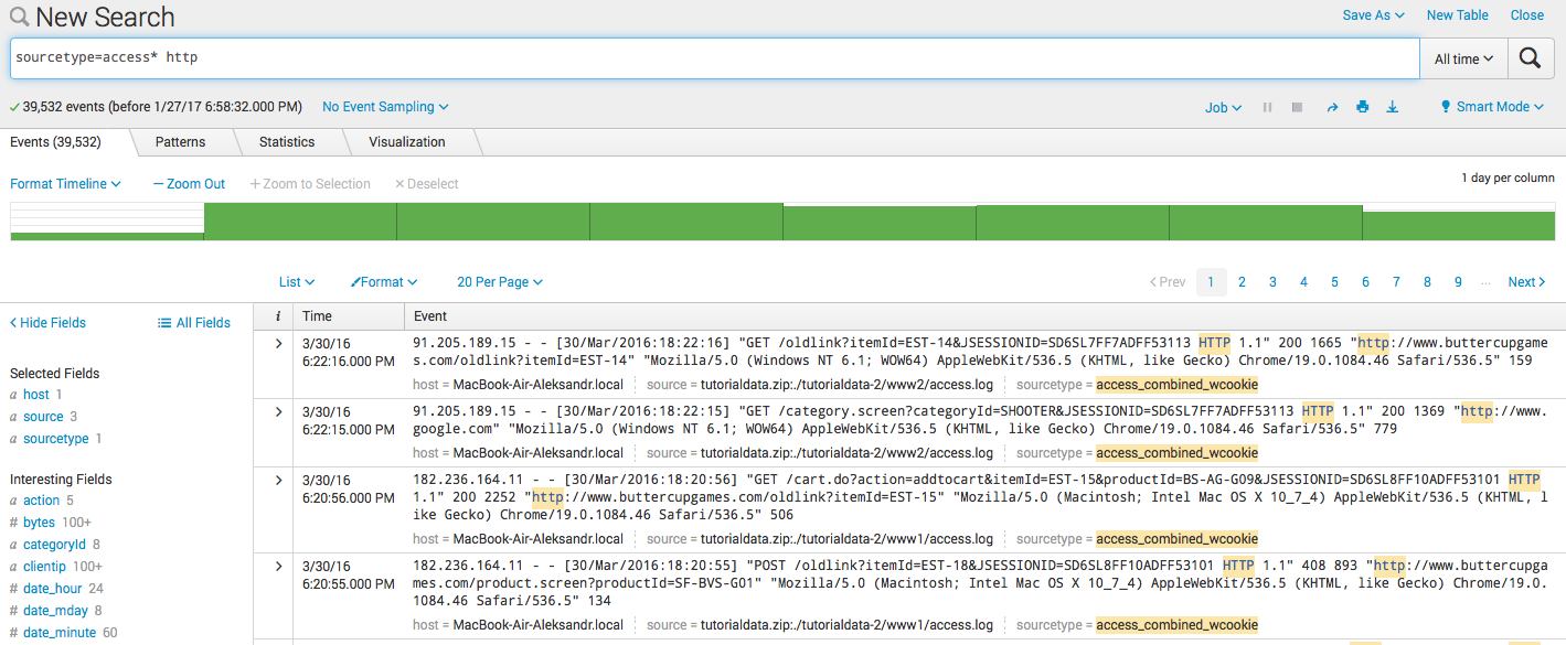
  
  
  
  
• Filtration : sourcetype = access * http clientip = 87.194.216.51
  
  
  
  
• Combination : sourcetype = access * http clientip = 87.194.216.51 (503 OR 504)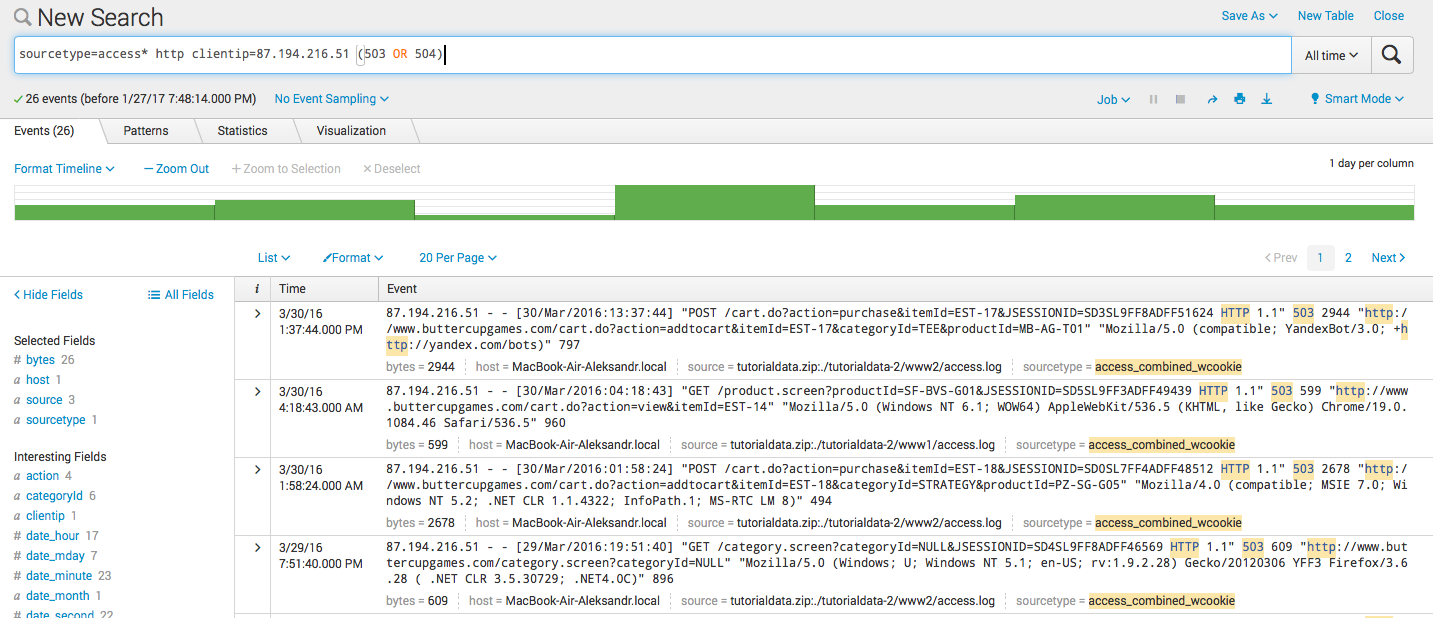
  
  
  

Calculated Fields (Eval):

Splunk can create new fields based on existing ones. For this, use the eval command, the syntax and example of which is described below. After we have created a field, it can also participate in further requests.

• Calculate new field: sourcetype = access * | eval KB = bytes / 1024
  
  
  
  
• Creating a new field by condition: sourcetype = access * | eval http_response = if (status! = 200, "Error", "OK")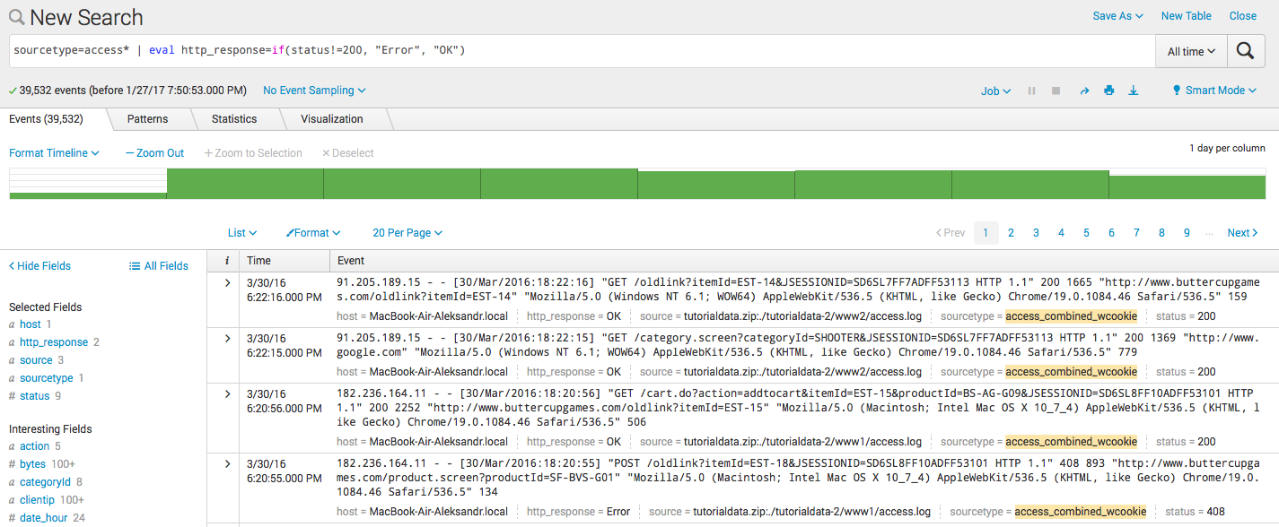
  
  
  
  
• Coupling two fields in the new: sourcetype = access * | eval connection = clientip. ":". other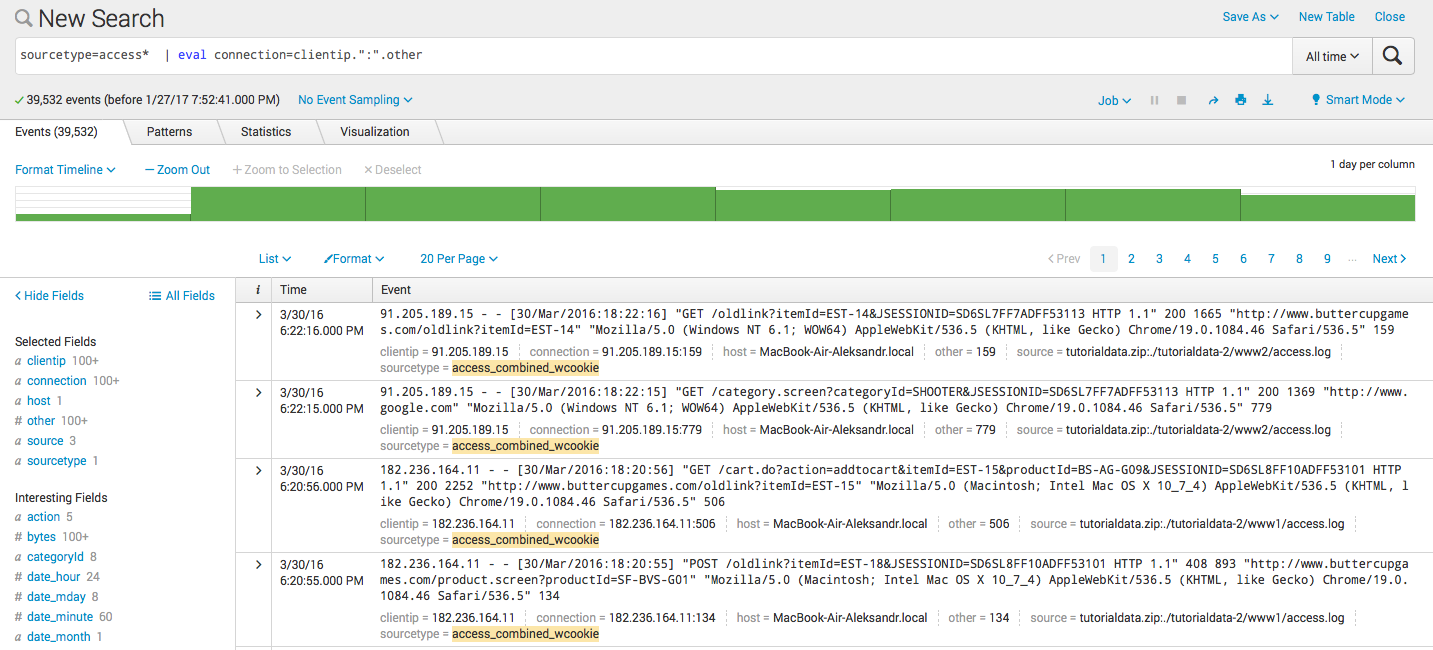
  
  

Statistical queries and visualization:

After we have learned to filter and create new fields, we proceed to the next stage - statistical queries or data aggregation. Plus, all this can naturally be visualized. For these requests, you will need to upload another test file to the system. It is important that at the download stage, change the sourcetype csv to eq using the Save As button, so that the results of the requests coincide with our screenshots.

• Calculation: sourcetype = "eq" | stats avg (mag) AS "Medium Magnitude"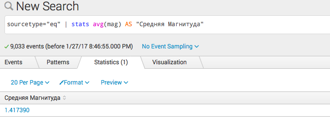
  
  
  
  
• Several calculations: sourcetype = "eq" | stats avg (mag) AS "Medium Magnitude", sparkline (avg (mag)) AS "Trend"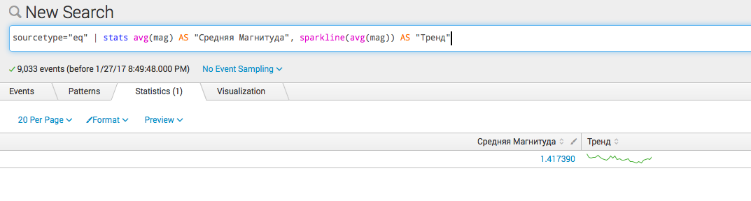
  
  
  
  
• Group by type sourcetype = "eq" | stats avg (mag) AS "Average Magnitude", sparkline (avg (mag)) AS "Trend" by type
  
  

Statistical queries in time:

Since Splunk performs all searches in time, one of the most common commands is timechart , which allows you to build statistical queries with reference to time, below are examples (you can choose the type of visualization in the interface under the statistics, visualization tabs and next to the format button):

• Visualization of simple time statistics: sourcetype = "eq" | timechart avg (mag) as "Medium magnitude"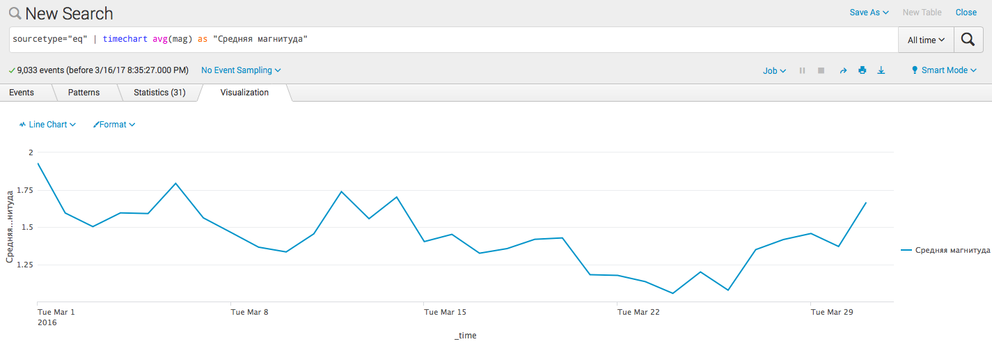
  
  
  
  
• Add a trend line ( algorithm ): sourcetype = "eq" | timechart avg (mag) as "Medium magnitude" | trendline sma5 ("Medium magnitude")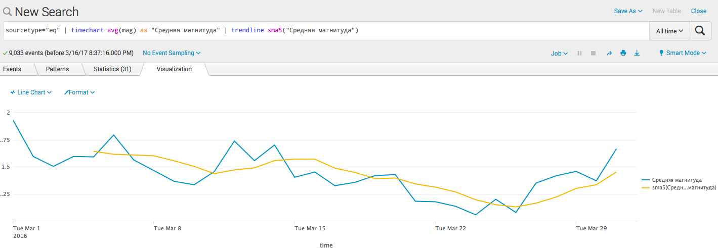
  
  
  
  
• Add predictive barriers: sourcetype = "eq" | timechart avg (mag) as "Medium magnitude" | predict "Average magnitude"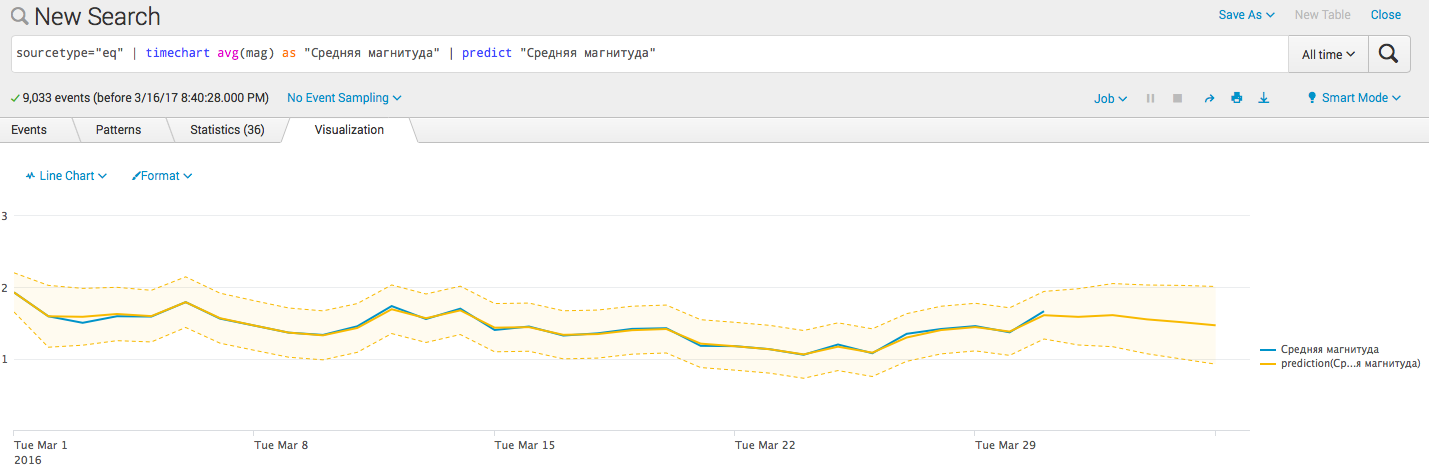
  
  

Conclusion

Next time we will talk about several interesting commands that allow you to work with data that has geographic coordinates and how and where to get these coordinates if they are not there, as well as grouping data to highlight transactions and identify the order of events.

I also want to note a super useful document containing in one place a lot of information about Splunk - Quick Reference Guide .