Another algorithm for recovering blurred images

Good day. Already so much has been said about the methods of deconvolution of images, it seems there is nothing more to add. However, there is always a better and newer algorithm than the previous ones. Not so long ago, an iterative algorithm was described, which has a linear convergence rate at low memory costs, is stable and well-parallelizable. And after a while it was improved even to quadratic convergence. Meet: (Fast) Iterative Shrinkage-Thresholding Algorithm.

Formulation of the problem

A long time ago a whole series of articles on image deconvolution algorithms was published. The cycle considered a classical method for solving systems of linear algebraic equations and their regularization. The described method, in terms of the formulation of the problem, is practically no different from the classical one, but the devil is in the details. Let's start our math magic. This is the classic expression of the received damaged and noisy image:

m a t h b f y = m a t h b f A x + m a t h b f n

$\ mathbf {y} = \ mathbf {Ax} + \ mathbf {n}$

')
Matrix

m a t h b f A

$\ mathbf {A}$ is a convolution matrix, and from a physical point of view it shows the relationship between the points of the original and the corrupted data. In the case of images, this matrix can be obtained by transforming the convolution kernel. Vectors

m a t h b f x

$\ mathbf {x}$ and

m a t h b f y

$\ mathbf {y}$ are the original and damaged image in vectorized form. In other words, all columns of pixels in an image are concatenated one by one.

The first problem of such a formulation of the problem: the amount of allocated memory. If the image has dimensions 640x480, then the task stores two vectors of images with dimensions of 307200x1 and a matrix of 307200x307200 elements. The convolution matrix is sparse, but its dimensions, even in a sparse form, will be large and will take a lot of memory. A product with a convolution matrix can be replaced with a two-dimensional convolution with the kernel, which does not require storing a large matrix in memory, this will solve the problem of storing the matrix

m a t h b f A

$\ mathbf {A}$ .
To search for the image as close as possible to the original one, we write the optimized function in the classical form of the second norm of the discrepancy between the damaged and the desired images.

m i n_{h a t m a t h b f x} m i d m i d m a t h b f y - A h a t x m i d m i d_{2}

$min _ {\ hat {\ mathbf {x}}} \ mid \ mid \ mathbf {y-A \ hat {x}} \ mid \ mid_2$

Difference from classical methods

This formulation of the problem is one of the most popular, but we will add to it to improve performance. The approach used is called “Majorization-maximization”, and it consists in replacing the original problem with another, very similar. The new task has two properties:

The task is much easier
At all points except the current one, there is a discrepancy greater than the original task.

This action occurs at each iteration of the algorithm. Sounds hard enough, much harder than it looks. Final minimization function for iteration

k

$k$ written as follows:

m a t h b f J_{k} (x) = m i d m i d m a t h b f y A h a t x m i d m i d_{2} + (m a t h b f h a t x - h a t x_{k})^{T} (a l p h a m a t h b f I - m a t h b f A^{T} A) (m a t h b f h a t x - h a t x_{k})

$\ mathbf {J_k (x)} = \ mid \ mid \ mathbf {yA \ hat {x}} \ mid \ mid_2 + (\ mathbf {\ hat {x} - \ hat {x_k}}) ^ T (\ alpha \ mathbf {I} - \ mathbf {A ^ TA}) (\ mathbf {\ hat {x} - \ hat {x_k}})$

The matrix of the right term is positive definite. This is achieved by the fact that

a l p h a > m a x e i g (m a t h b f A^{T} A)

$\ alpha> maxeig (\ mathbf {A ^ TA})$ . The minimization function consists of the sum of two quantities, each of which is non-negative. At the same time, at the point

m a t h b f h a t x = h a t x_{k}

$\ mathbf {\ hat {x} = \ hat {x} _k}$ the second term is zero, due to which the second condition from the list is satisfied.

Finding a solution

We will begin the search for a solution using the classical method: open the brackets, write out the gradient and equate it to zero. It is important to notice this gradient on

k

$k$ iteration Attention a lot of math!

m a t h b f J_{k} (h a t x) = (m a t h b f y A h a t x)^{T} (m a t h b f y A h a t x) + (m a t h b f h a t x - h a t x_{k})^{T} c d o t (a l p h a m a t h b f I - m a t h b f A^{T} A) c d o t (m a t h b f h a t x - h a t x_{k})

$\ mathbf {J_k (\ hat {x})} = (\ mathbf {yA \ hat {x}}) ^ T (\ mathbf {yA \ hat {x}}) + (\ mathbf {\ hat {x} - \ hat {x} _k}) ^ T \ cdot (\ alpha \ mathbf {I} - \ mathbf {A ^ TA}) \ cdot (\ mathbf {\ hat {x} - \ hat {x} _k})$

m a t h b f J_{k} (h a t x) = m a t h b f y^{T} y + m a t h b f h a t x^{T} A^{T} A h a t x - 2 m a t h b f y^{T} A h a t x - - m a t h b f h a t x^{T} (a l p h a m a t h b f I - m a t h b f A^{T} A) h a t x + m a t h b f h a t x_{k}^{T} (a l p h a m a t h b f I - m a t h b f A^{T} A) h a t x_{k} - 2 m a t h b f h a t x_{k}^{T} (a l p h a m a t h b f I - m a t h b f A^{T} A) h a t x

$\ mathbf {J_k (\ hat {x})} = \ mathbf {y ^ Ty} + \ mathbf {\ hat {x} ^ TA ^ TA \ hat {x}} -2 \ mathbf {y ^ TA \ hat {x}} - \\ - \ mathbf {\ hat {x} ^ T (\ alpha \ mathbf {I} - \ mathbf {A ^ TA}) \ hat {x}} + \ mathbf {\ hat {x} _k ^ T (\ alpha \ mathbf {I} - \ mathbf {A ^ TA}) \ hat {x} _k} -2 \ mathbf {\ hat {x} _k ^ T (\ alpha \ mathbf {I} - \ mathbf {A ^ TA}) \ hat {x}}$

f r a c m a t h b f J_{k} (h a t x) d e l t a m a t h b f h a t x = m a t h b f A^{T} A h a t x - 2 m a t h b f A^{T} y + m a t h b f 2 a l p h a m a t h b f I h a t x - m a t h b f A^{T} A h a t x - 2 m a t h b f (a l p h a m a t h b f I - m a t h b f A^{T} A) h a t x_{k}

$\ frac {\ mathbf {J_k (\ hat {x})}} {\ delta \ mathbf {\ hat {x}}} = \ mathbf {A ^ TA \ hat {x}} -2 \ mathbf {A ^ Ty} + \ mathbf {2 \ alpha \ mathbf {I} \ hat {x} - \ mathbf {A ^ TA} \ hat {x}} - 2 \ mathbf {(\ alpha \ mathbf {I} - \ mathbf { A ^ TA}) \ hat {x} _k}$

As a result, the derivative will have the following form:

d e l t a J_{k} (x) = 2 m a t h b f A^{T} y - 2 (a l p h a m a t h b f I A^{T} A) m a t h b f h a t x_{k} + 2 a l p h a m a t h b f h a t x

$\ delta J_k (x) = 2 \ mathbf {A ^ Ty} -2 (\ alpha \ mathbf {IA ^ TA}) \ mathbf {\ hat {x} _k} +2 \ alpha \ mathbf {\ hat {x }}$

The next classical step in this situation is to equate the gradient to zero, and express the desired vector from the resulting expression.

m a t h b f h a t x

$\ mathbf {\ hat {x}}$ . Recorded

m a t h b f h a t x

$\ mathbf {\ hat {x}}$ we define as

m a t h b f h a t x_{n + 1}

$\ mathbf {\ hat {x} _ {n + 1}}$ or as a solution at the next iteration.

d e l t a J_{k} (x) = 2 m a t h b f A^{T} y - 2 (a l p h a m a t h b f I A^{T} A) m a t h b f h a t x_{k} + 2 a l p h a m a t h b f h a t x = 0

$\ delta J_k (x) = 2 \ mathbf {A ^ Ty} -2 (\ alpha \ mathbf {IA ^ TA}) \ mathbf {\ hat {x} _k} +2 \ alpha \ mathbf {\ hat {x }} = 0$

m a t h b f A^{T} y + a l p h a m a t h b f I m a t h b f h a t x_{k} - m a t h b f A^{T} A m a t h b f h a t x_{k} = a l p h a m a t h b f h a t x

$\ mathbf {A ^ Ty} + \ alpha \ mathbf {I} \ mathbf {\ hat {x} _k} - \ mathbf {A ^ TA} \ mathbf {\ hat {x} _k} = \ alpha \ mathbf { \ hat {x}}$

m a t h b f h a t x_{k + 1} = m a t h b f h a t x_{k} + f r a c 1 a l p h a c d o t m a t h b f A^{T} (y A h a t x_{k})

$\ mathbf {\ hat {x} _ {k + 1}} = \ mathbf {\ hat {x} _k} + \ frac {1} {\ alpha} \ cdot \ mathbf {A ^ T (yA \ hat { x_k})}$

The resulting expression is called "Landweber iteration". This is the basic formula between iterations. Using it, you can guarantee a decrease in the discrepancy from iteration to iteration with a linear velocity.

The basic algorithm contains an additional step, called “soft-threshold”, and implying sparseness of the solution. This step equates to zero all the values of the desired vector modulo smaller than the set value. This reduces the impact of noise on the recovery result.

What it looks like

As can be seen from the decision, we have two parameters that we adjust to our taste.

l a m b d a

$\ lambda$ responsible for the accuracy of the approximation, limiting the convergence of the threshold.

a l p h a

$\ alpha$ is responsible for the stability of work and the rate of convergence of the algorithm.

m a t h b f h a t x_{k + 1} = s o f t (m a t h b f h a t x_{k} + f r a c 1 a l p h a c d o t m a t h b f A^{T} (y A h a t x_{k}), l a m b d a / a l p h a)

$\ mathbf {\ hat {x} _ {k + 1}} = soft (\ mathbf {\ hat {x} _k} + \ frac {1} {\ alpha} \ cdot \ mathbf {A ^ T (yA \ hat {x_k})}, \ lambda / \ alpha)$

Algorithm modification

In the future, the algorithm was improved by an additional term, similar in theory to the conjugate gradient method. Adding at each step the difference between the result of the two previous iterations, we increase the convergence of the algorithm to quadratic. The final procedure of the algorithm is as follows:

Set parameters $\ lambda, \ alpha$
Set $t_1 = 1, t_0 = 1, \ mathbf {y_ {temp} = \ hat {x} _0 = A ^ Ty}$
Iterate the base algorithm $\ mathbf {\ hat {x} _ {k + 1}} = soft (\ mathbf {y_ {temp}} + \ frac {1} {\ alpha} \ cdot \ mathbf {A ^ T (y-Ay_ { temp})}, \ lambda / \ alpha)$
Update Temporary Variables
$t_0 = t_1; t_1 = 0.5 + \ sqrt {0.25 + t_1 ^ 2}$
Add a conjugate component to a variable $\ mathbf {y_ {temp} = \ hat {x} _k} + \ frac {t_0-1} {t_1} \ cdot (\ mathbf {\ hat {x} _k- \ hat {x} _ {k-1 }})$

Now about the parallelism of the algorithm. The cycle for calculating the threshold at each iteration can be expressed through elementwise products (Hadamard product) and comparison operations, which are included in both OpenCL and CUDA, so that they can be easily parallelized.

I implemented the algorithm on Matlab in two versions: for computing on the CPU and on the GPU. Later I began to use only the version of the code for the GPU, since it is more convenient. The code is presented below.

Code here

function [x] = fista_gpu(y,H,Ht,lambda,alpha,Nit) x=Ht(y); y_k=x; t_1=1; T=lambda/alpha; for k = 1:Nit x_old=x; x=soft_gpu((y_k+(1/alpha)*Ht(yH(y_k))), T); t_0=t_1-1; t_1=0.5+sqrt(0.25+t_1^2); y_k=x+(t_0/t_1)*(x-x_old); end end function [y] = soft_gpu(x,T) eq=ge(abs(x),abs(T)); y=eq.*sign(x).*(abs(x)-abs(T)); end

Let's go down closer to the practice, and test the performance of the algorithm depending on the size of the picture.

My laptop configuration

Intel core I3-4005U
NVIDIA GeForce 820M

On the left is a graph of the dependence of the algorithm on 100 iterations, depending on the number of pixels for the CPU and GPU.

As can be seen from the results, the algorithm on the GPU is practically independent of the size of the task and for really large images we are limited only by the GPU memory. Half a second for 2000x2000 (without taking into account the unloading from memory) is a decent result, isn't it?
The right is the dependence of the time spent by the algorithm on the number of iterations. As the number of iterations increases, the algorithm on the GPU begins to respond by increasing the runtime. Most likely, this is due to my mistakes in writing code, or the forced lowering of the frequency of the GPU. In most cases, 100 iterations are enough.

The following graphs present a comparison of the basic and improved algorithm, as well as the dependence of the algorithm’s convergence on

a l p h a

$\ alpha$ and

l a m b d a

$\ lambda$ parameters.

As can be seen from the graph on the left, the improved algorithm converges much faster than the baseline, and after one hundred iterations it practically does not show an increase in accuracy. The basic algorithm only to the five-hundredth iteration shows an acceptable result.
According to the central schedule can be seen, depending on $\ lambda$ the convergence threshold of the algorithm changes, which limits performance. This is a necessary compromise if the signal is very noisy.
On the right graph shows that with increasing $\ alpha$ the algorithm converges much slower. Similar to the previous case, there is a compromise between the "quality" of the convolution matrix and the rate of convergence.

And finally, an example of the algorithm on the FHD picture,

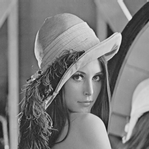
Source picture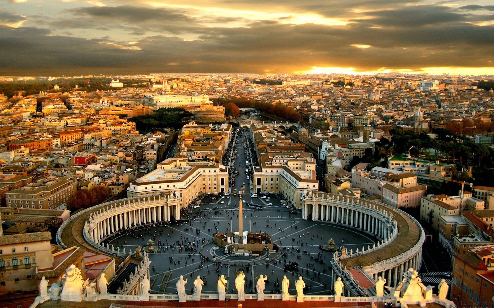

Corroded and Noisy Picture

Recovered picture

As you can see, the result is quite good, especially if it takes only 15 seconds, of which 1.5 is the work of the algorithm and 13.5 uploading a picture from the GPU memory.
All the code used for the algorithm is laid out in GitHub .

References

I. Selesnick. (2009) About: Sparse signal restoration.
A. Beck and M. Teboulle Fast Gradient-Based Algorithms for Constrained Total Variation Image IEEE TRANSACTIONS ON IMAGE PROCESSING, VOL. 18, NO. 11, NOVEMBER 2009
PL Combettes and J.-C. Pesquet Proximal Splitting Methods in Signal Processing

Source: https://habr.com/ru/post/324052/

All Articles