Hello!

Today we will discuss in detail a very important class of machine learning models - linear. The key difference between our presentation of the material from similar econometrics and statistics in the courses is an emphasis on the practical application of linear models in real problems (although there will be plenty of mathematics too).

An example of such a task is the Kaggle Inclass competition for identifying a user on the Internet by his site navigation sequence.

UPD: now the course is in English under the brand mlcourse.ai with articles on Medium, and materials on Kaggle ( Dataset ) and on GitHub .

All materials are available on GitHub .
And here is a video of a lecture based on this article as part of the second launch of the open course (September-November 2017). In particular, it considers two benchmark competitions obtained using logistic regression.

Plan for this article:

1. Linear regression
   
   • Least square method
   • Maximum Likelihood Method
   • Decomposition of an error into displacement and spread (Bias-variance decomposition)
   • Regularization of linear regression
2. Logistic regression
   
   • Linear Classifier
   • Logistic regression as a linear classifier
   • Maximum Likelihood Principle and Logistic Regression
   • L2-regularization of logistic loss function
3. A good example of the regularization of logistic regression
4. Where logistic regression is good and where not so
   - Analysis of IMDB movie reviews
   - XOR problem
5. Validation and training curves
6. Pros and cons of linear models in machine learning problems
7. Homework number 4
8. Useful resources

1. Linear regression

Least square method

We begin the story about linear models with linear regression. First of all, it is necessary to set the model of dependence of the explained variable $$$y$ from the factors explaining it, the dependency function will be linear: $$$y = w_0 + \ sum_ {i = 1} ^ m w_i x_i$ . If we add a dummy dimension $$$x_0 = 1$ for each observation, then the linear form can be rewritten a little more compactly by writing the free term $$$w_0$ under the amount of: $$$y = \ sum_ {i = 0} ^ m w_i x_i = \ vec {w} ^ T \ vec {x}$ . If we consider the observation-features matrix, in which there are examples from the data set in the rows, we need to add a single column to the left. Set the model as follows:

Where

• $$$\ vec y \ in \ mathbb {R} ^ n$ - explainable (or target) variable;
• $$$w$ - vector of model parameters (in machine learning, these parameters are often called weights);
• $$$X$ - matrix of observations and signs of dimension $$$n$ rows on $$$m + 1$ columns (including a dummy single column on the left) with full column rank: $$$\ text {rank} \ left (X \ right) = m + 1$ ;
• $$$\ epsilon$ - random variable corresponding to a random, unpredictable model error.

We can write the expression for each specific observation

Also, the following restrictions are imposed on the model (otherwise it will be some other regression, but definitely not linear):

• The expectation of random errors is zero: $$$\ forall i: \ mathbb {E} \ left [\ epsilon_i \ right] = 0$ ;
• the variance of random errors is the same and finite, this property is called homoscedasticity : $$$\ forall i: \ text {Var} \ left (\ epsilon_i \ right) = \ sigma ^ 2 <\ infty$ ;
• random errors are not correlated: $$$\ forall i \ neq j: \ text {Cov} \ left (\ epsilon_i, \ epsilon_j \ right) = 0$ .

Evaluation $$$\ hat {w} _i$ weights $$$w_i$ called linear if

Where $$$\ forall \ k \ \ omega_ {ki}$ depends only on the observed data $$$X$ and almost certainly nonlinear. Since the linear estimation is the solution to the problem of finding the optimal weights, the model is also called a linear regression . We introduce another definition. Evaluation $$$\ hat {w} _i$ is called unbiased when the expectation of the estimate is equal to the real, but unknown value of the estimated parameter:

One way to calculate the values ​​of the model parameters is the least squares method (OLS), which minimizes the root-mean-square error between the real value of the dependent variable and the forecast given by the model:

To solve this optimization problem, it is necessary to calculate the derivatives with respect to the model parameters, equate them to zero and solve the resulting equations for $$$\ vec w$ (Matrix differentiation may seem inconvenient to an unprepared reader, try writing through all the amounts to make sure of the answer):

So, bearing in mind all the definitions and conditions described above, we can argue, based on the Markov-Gauss theorem , that the LSM estimate is the best estimate of the model parameters, among all linear and unbiased estimates, that is, having the least variance.

Maximum Likelihood Method

The reader could reasonably have questions: for example, why do we minimize the root-mean-square error, and not something else? After all, you can minimize the average absolute value of the residual or something else. The only thing that happens in case of a change in the minimized value is that we will leave the conditions of the Markov-Gauss theorem, and our estimates will cease to be the best among linear and unbiased.

Before continuing, let us make a lyrical digression to illustrate the maximum likelihood method using a simple example.

Once after school, I noticed that everyone remembers the formula of ethyl alcohol. Then I decided to conduct an experiment: do people remember the simpler formula of methyl alcohol: $$$CH_3OH$ . We interviewed 400 people and it turned out that only 117 people remember the formula. It is reasonable to assume that the probability that the next respondent knows the formula of methyl alcohol - $$$\ frac {117} {400} \ approx 0.29%$ . We show that such an intuitive assessment is not just good, but also an estimate of maximum likelihood.

Let us see where this estimate comes from, and for this we recall the definition of the Bernoulli distribution : a random variable $$$X$ has a Bernoulli distribution if it takes only two values ​​( $$$1$ and $$$0$ with probabilities $$$\ theta$ and $$$1 - \ theta$ respectively) and has the following probability distribution function:

It looks like this distribution is what we need, and the distribution parameter $$$\ theta$ and there is that estimate of the probability that a person knows the formula of methyl alcohol. We have done $$$400$ independent experiments, we denote their outcomes as $$$\ vec {x} = \ left (x_1, x_2, \ ldots, x_ {400} \ right)$ . Let's write down the credibility of our data (observations), that is, the probability of observing 117 realizations of a random variable $$$X = 1$ and 283 implementations $$$X = 0$ :

Next, we will maximize this expression by $$$\ theta$ and most often this is not done with credibility $$$p (\ vec {x} \ mid \ theta)$ , and with its logarithm (applying a monotone transform will not change the solution, but will simplify the calculations):

Now we want to find such a value. $$$\ theta$ which maximizes likelihood, for this we take the derivative with respect to $$$\ theta$ , equate to zero and solve the resulting equation:

It turns out that our intuitive assessment is the maximum likelihood estimate. We now apply the same reasoning for the linear regression problem and try to find out what lies behind the root-mean-square error. To do this, we will have to look at linear regression from a probabilistic point of view. The model naturally remains the same:

but we will now assume that random errors are taken from the centered normal distribution :

Rewrite the model in a new light:

Since examples are taken independently (errors are not correlated — one of the conditions of the Markov – Gauss theorem), the full likelihood of the data will look like a product of density functions $$$p \ left (y_i \ right)$ . Consider the logarithm of the likelihood, which will allow us to move from product to sum:

We want to find the maximum likelihood hypothesis, i.e. we need to maximize expression $$$p \ left (\ vec {y} \ mid X, \ vec {w} \ right)$ , and this is the same as maximizing its logarithm. Note that when maximizing a function with a parameter, you can throw out all the members that are independent of this parameter:

Thus, we have seen that maximizing the likelihood of data is the same as minimizing the root-mean-square error (with the validity of the above assumptions). It turns out that precisely such a cost function is a consequence of the fact that the error is distributed normally, and not in any other way.

Decomposition of an error into displacement and spread (Bias-variance decomposition)

Let's talk a little about the properties of the linear regression prediction error (in principle, these arguments are true for all machine learning algorithms). In light of the previous paragraph, we found that:

• the true value of the target variable is made up of some deterministic function $$$f \ left (\ vec {x} \ right)$ and random error $$$\ epsilon$ : $$$y = f \ left (\ vec {x} \ right) + \ epsilon$ ;
• the error is distributed normally with a center at zero and some variation: $$$\ epsilon \ sim \ mathcal {N} \ left (0, \ sigma ^ 2 \ right)$ ;
• the true value of the target variable is also distributed normally: $$$y \ sim \ mathcal {N} \ left (f \ left (\ vec {x} \ right), \ sigma ^ 2 \ right)$
• we are trying to bring a deterministic but unknown function $$$f \ left (\ vec {x} \ right)$ linear function of regressors $$$\ hat {f} \ left (\ vec {x} \ right)$ which in turn is a point estimate of the function $$$f$ in the space of functions (more precisely, we restricted the space of functions to the parametric family of linear functions), i.e. random variable, which has a mean and variance.

Then the error is at the point $$$\ vec {x}$ decomposed as follows:

For clarity, we omit the designation of the argument of functions. Consider each member individually, the first two are easily painted by the formula $$$\ text {Var} \ left (z \ right) = \ mathbb {E} \ left [z ^ 2 \ right] - \ mathbb {E} \ left [z \ right] ^ 2$ :

Explanations:

And now the last member of the amount. We remember that the error and the target variable are independent of each other:

Finally, we put everything together:

So, we have achieved the goal of all the calculations described above, the last formula tells us that the prediction error of any model of the type $$$y = f \ left (\ vec {x} \ right) + \ epsilon$ composed of:

• offset square: $$$\ text {Bias} \ left (\ hat {f} \ right)$ - the average error for all sorts of data sets;
• dispersion: $$$\ text {Var} \ left (\ hat {f} \ right)$ - error variability, then how much the error will differ if you train the model on different data sets;
• Fatal error: $$$\ sigma ^ 2$ .

If we cannot do anything with the latter, then we can somehow influence the first two terms. Ideally, of course, I would like to negate both of these terms (the upper left square of the figure), but in practice it is often necessary to balance between biased and unstable estimates (high variance).

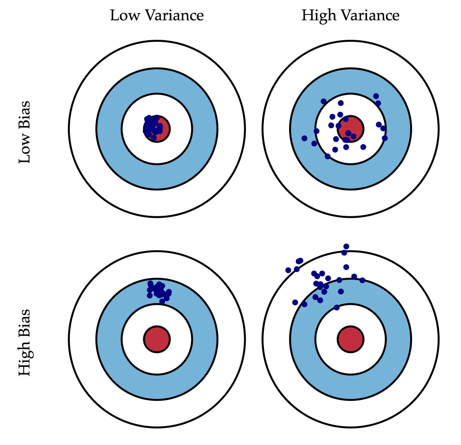
As a rule, as the model complexity increases (for example, as the number of free parameters increases), the variance (scatter) of the estimate increases, but the offset decreases. Due to the fact that the training data set is fully remembered instead of generalized, small changes lead to unexpected results (retraining). If the model is weak, then it is not able to learn the pattern, as a result, something else is learned that is shifted relative to the correct solution.

The Markov-Gauss theorem asserts that the least-squares estimate of the parameters of a linear model is the best in the class of unbiased linear estimates, that is, with the least variance. This means that if there is any other unbiased model $$$g$ also from the class of linear models, then we can be sure that $$$Var \ left (\ hat {f} \ right) \ leq var \ left (g \ right)$ .

Regularization of linear regression

Sometimes there are situations when we intentionally increase the bias of the model for the sake of its stability, i.e. to reduce the dispersion of the model $$$\ text {Var} \ left (\ hat {f} \ right)$ . One of the conditions of the Markov – Gauss theorem is the full column rank of the matrix $$$X$ . Otherwise, the MNC solution $$$\ vec {w} = \ left (X ^ T X \ right) ^ {- 1} X ^ T \ vec {y}$ does not exist, because there will be an inverse matrix $$$\ left (X ^ T X \ right) ^ {- 1}.$ In other words, the matrix $$$X ^ t x$ will be singular or degenerate. This task is called incorrectly set . The task needs to be corrected, namely, to make the matrix $$$X ^ tx$ non-degenerate, or regular (which is why this process is called regularization). More often in the data we can observe the so-called multicollinearity - when two or more signs are strongly correlated, in the matrix $$$X$ this manifests itself in the form of a “almost” linear dependence of the columns. For example, in the task of forecasting the price of an apartment according to its parameters, “almost” linear dependence will have signs “area with balcony” and “area without balcony”. Formally, for such data the matrix $$$X ^ t x$ will be reversible, but because of the multicollinearity of the matrix $$$X ^ t x$ some eigenvalues ​​will be close to zero, and in the inverse matrix $$$\ left (X ^ T X \ right) ^ {- 1}$ Extremely large eigenvalues ​​will appear, since inverse matrix eigenvalues ​​are $$$\ frac {1} {\ lambda_i}$ . The result of such a reel of eigenvalues ​​will be an unstable estimate of the model parameters, i.e. adding a new observation to the training data set will lead to a completely different solution. Illustrations of the growth of the ratios can be found in one of our past posts . One of the regularization methods is Tikhonov regularization , which, in general, looks like the addition of a new term to the root-mean-square error:

Often the Tikhonov matrix is ​​expressed as the product of a certain number by the identity matrix: $$$\ Gamma = \ frac {\ lambda} {2} E$ . In this case, the problem of minimizing the root-mean-square error becomes a problem with a constraint on $$$L_2$ the norm. If we differentiate the new function of cost by the parameters of the model, equate the resulting function to zero and express $$$\ vec {w}$ then we get the exact solution to the problem.

This regression is called ridge regression. And the crest is just the diagonal matrix, which we add to the matrix $$$X ^ t x$ , the result is a guaranteed regular matrix.

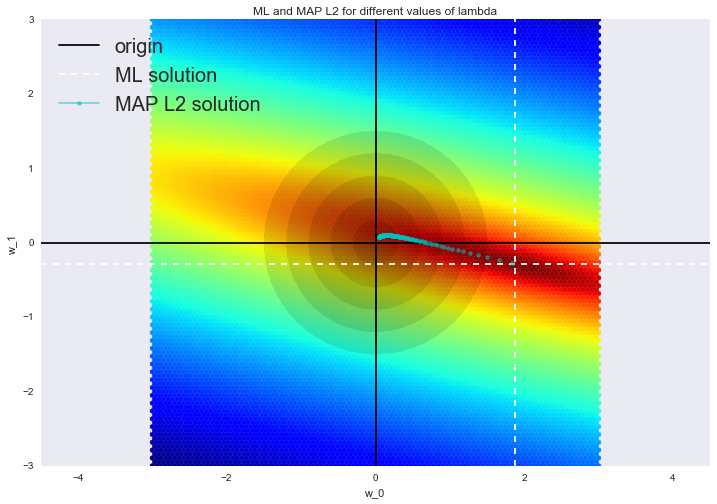
Such a solution reduces the variance, but becomes biased, since the norm of the parameter vector is also minimized, which causes the solution to shift towards zero. The figure below at the intersection of white dotted lines is the OLS-solution. Blue dots indicate different ridge regression solutions. It is seen that with an increase in the regularization parameter $$$\ lambda$ the solution shifts towards zero.

We advise you to contact our last post for an example of how $$$L_2$ regularization cope with the problem of multicollinearity, as well as to refresh a few more interpretations of regularization.

2. Logistic regression

Linear Classifier

The basic idea of ​​a linear classifier is that the feature space can be divided by the hyperplane into two half-spaces, in each of which one of the two values ​​of the target class is predicted.
If this can be done without errors, then the training set is called linearly separable .

We are already familiar with linear regression and the least squares method. Consider the problem of binary classification, with labels of the target class denoted by "+1" (positive examples) and "-1" (negative examples).
One of the simplest linear classifiers is obtained on the basis of a regression like this:

Where

• $$$\ vec {x}$ - vector of example signs (together with the unit);
• $$$\ vec {w}$ - weights in a linear model (along with an offset $$$w_0$ );
• $$$sign (\ bullet)$ - Signum function, returning the sign of its argument;
• $$$a (\ vec {x})$ - classifier response by example $$$\ vec {x}$ .

Logistic regression as a linear classifier

Logistic regression is a particular case of a linear classifier, but it has a good “ability” to predict the probability $$$p _ +$ example assignments $$$\ vec {x_i}$ to class "+":

Prediction is not just an answer ("+1" or "-1"), namely the probability of being assigned to the class "+1" in many tasks is a very important business requirement. For example, in the problem of credit scoring, where logistic regression is traditionally used, the probability of loan default is often predicted ( $$$p _ +$ ). Clients who apply for a loan are sorted according to this predicted probability (descending), and the result is a scoring map - in fact, the rating of clients from bad to good. Below is a toy example of such a scart card.

The bank chooses for itself the threshold $$$p _ *$ predicted probability of loan default (in the picture - $$$0.15$ ) and starting from this value no longer issues a loan. Moreover, you can multiply the predicted probability by the amount issued and get the expectation of losses from the client, which will also be a good business metric ( Further in the comments, scoring experts can fix it, but the main point is something like this ).

So we want to predict the probability $$$p_ + \ in [0,1]$ but for now we are able to build a linear forecast using the OLS: $$$b (\ vec {x}) = \ vec {w} ^ T \ vec {x} \ in \ mathbb {R}$ . How to convert the resulting value into a probability whose limits are [0, 1]? Obviously, this requires some function. $$$f: \ mathbb {R} \ rightarrow [0,1].$ In the logistic regression model, a specific function is taken for this: $$$\ sigma (z) = \ frac {1} {1 + \ exp ^ {- z}}$ . And now we will understand what are the prerequisites for this.

Denote $$$P (x)$ probability of an event occurring $$$X$ . Then the ratio of probabilities $$$OR (X)$ determined from $$$\ frac {P (X)} {1-P (X)}$ , and this is the ratio of the probabilities of whether an event will occur or not. It is obvious that probability and odds ratio contain the same information. But while $$$P (x)$ ranges from 0 to 1, $$$OR (X)$ ranges from 0 to $$$\ infty$ .

If you calculate the logarithm $$$OR (X)$ (that is, it is called the logarithm of odds, or the logarithm of the ratio of probabilities), it is easy to notice that $$$\ log {OR (X)} \ in \ mathbb {R}$ . Its something we will predict using OLS.

Let's see how logistic regression will predict $$$p_ + = P \ left (y_i = 1 \ mid \ vec {x_i}, \ vec {w} \ right)$ (while we consider that weights $$$\ vec {w}$ we somehow got it (ie, we trained the model), then we'll figure out how exactly).

• Step 1. Calculate the value. $$$w_ {0} + w_ {1} x_1 + w_ {2} x_2 + ... = \ vec {w} ^ T \ vec {x}$ . (the equation $$$\ vec {w} ^ T \ vec {x} = 0$ sets a hyperplane, dividing the examples into 2 classes);

  
  

• Step 2. Calculate the log odds ratio: $$$\ log (OR _ {+}) = \ vec {w} ^ T \ vec {x}$ .

  
  

• Step 3. Having a prediction of the chances of being classified as "+" - $$$OR _ {+}$ compute $$$p _ {+}$ using a simple dependency:

  
  

In the right-hand side, we got just the sigmoid function.

So, the logistic regression predicts the probability of attributing an example to the “+” class (provided that we know its characteristics and model weights) as a sigmoid transformation of a linear combination of the model weights vector and example vector characteristics:

The next question is: how is the model being trained? Here we again appeal to the principle of maximum likelihood.

Maximum Likelihood Principle and Logistic Regression

Now let's see how the maximum likelihood principle results in an optimization problem that the logistic regression solves, namely, minimization of the logistic loss function.
We have just seen that logistic regression models the probability of classifying an example to the class “+” as

Then for the class "-" a similar probability:

Both of these expressions can be cleverly combined into one (watch my hands - do you not deceive you):

Expression $$$M (\ vec {x_i}) = y_i \ vec {w} ^ T \ vec {x_i}$ called indent ( margin ) classification on the object $$$\ vec {x_i}$ (not to be confused with the gap (also the margin), about which they most often speak in the context of SVM). If it is non-negative, the model does not make a mistake on the object. $$$\ vec {x_i}$ if negative, then the class for $$$\ vec {x_i}$ predicted wrong.
Note that the indent is defined for the objects of the training sample for which the actual labels of the target class are known. $$$y_i$ .

To understand why we made such conclusions, let us turn to the geometric interpretation of the linear classifier. Details about this can be found in the materials of Yevgeny Sokolov.

I recommend to solve the almost classical problem from the initial course of linear algebra: find the distance from the point with the radius vector $$$\ vec {x_A}$ to the plane, which is given by the equation $$$\ vec {w} ^ T \ vec {x} = 0.$

When we receive (or see) the answer, we will understand that the more modulo the expression $$$\ vec {w} ^ T \ vec {x_i}$ the farther point $$$\ vec {x_i}$ is off the plane $$$\ vec {w} ^ T \ vec {x} = 0.$

Mean expression $$$M (\ vec {x_i}) = y_i \ vec {w} ^ T \ vec {x_i}$ - this is a kind of "confidence" model in the classification of the object $$$\ vec {x_i}$ :

• if the indent is large (by module) and positive, it means that the class label is set correctly, and the object is far from the separating hyperplane (such an object is classified confidently). On the picture - $$$x_3$ .
• if the indent is large (modulo) and negative, then the class label is set incorrectly, and the object is far from the separating hyperplane (most likely such an object is an anomaly, for example, its label in the training set is set incorrectly). On the picture - $$$x_1$ .
• if the indent is small (by module), then the object is close to the separating hyperplane, and the indentation sign determines whether the object is correctly classified. On the picture - $$$x_2$ and $$$x_4$ .

Now we shall write out the likelihood of the sample, namely, the probability of observing this vector $$$\ vec {y}$ have a sample $$$X$ . We make a strong assumption: objects come independently, from one distribution ( iid ). Then

Where $$$\ ell$ - sample length $$$X$ (number of lines).

As usual, let's take the logarithm of this expression (the sum is much easier to optimize than the product):

That is, in this case, the principle of maximizing the likelihood leads to minimization of the expression

This is a logistic loss function, summed over all objects of the training sample.

Let's look at the new function as a function of the indent: $$$L (M) = \ log (1 + \ exp ^ {- M})$ . Let's draw its schedule, and also the schedule of 1/0 loss function ( zero-one loss ), which simply penalizes the model for 1 for an error on each object (negative indent): $$$L_ {1/0} (M) = [M <0]$ .

The picture reflects the general idea that in the classification task, not being able to directly minimize the number of errors (at least, gradient methods do not do this - the derivative of 1/0 loss function at zero goes to infinity), we minimize some of its upper bound. In this case, it is the logistic loss function (where the logarithm is binary, but this is not critical), and

Where $$$\ mathcal {L_ {1/0}} (X, \ vec {y}, \ vec {w})$ - simply the number of logistic regression errors with weights $$$\ vec {w}$ on the sample $$$(X, \ vec {y})$ .

That is, reducing the top score $$$\ mathcal {L_ {log}}$ by the number of classification errors, we thus hope to reduce the number of errors itself.

$$$L_2$ -regularization of logistic losses

L2-regularization of logistic regression is arranged in almost the same way as in the case of ridge (Ridge regression). Instead of functional $$$\ mathcal {L_ {log}} (X, \ vec {y}, \ vec {w})$ minimizes the following:

In the case of logistic regression, the introduction of the inverse regularization coefficient is assumed. $$$C = \ frac {1} {\ lambda}$ . And then the solution will be

Next, consider an example that allows you to intuitively understand one of the meanings of regularization.

3. A good example of the regularization of logistic regression

In article 1, an example was given of how polynomial features allow linear models to construct nonlinear separating surfaces. Let's show it in pictures.

Let us see how regularization affects the quality of the classification on the data set for testing microchips from the Andrew Ng machine learning course.
We will use logistic regression with polynomial features and vary the regularization parameter C.
First, we will look at how regularization affects the classifier dividing border, intuitively recognize re-training and under-training.
Then, we numerically establish a near-optimal regularization parameter using cross validation (cross-validation) and iterating over the grid (GridSearch).

from __future__ import division, print_function #    Anaconda import warnings warnings.filterwarnings('ignore') %matplotlib inline from matplotlib import pyplot as plt import seaborn as sns import numpy as np import pandas as pd from sklearn.preprocessing import PolynomialFeatures from sklearn.linear_model import LogisticRegression, LogisticRegressionCV from sklearn.model_selection import cross_val_score, StratifiedKFold from sklearn.model_selection import GridSearchCV 

Load the data using the pandas read_csv method. In this data set for 118 microchips (objects), the results of two quality control tests (two numerical characters) are shown and it is said whether the microchip was put into production. The signs are already centered, that is, the column averages are subtracted from all values. Thus, the "average" microchip corresponds to zero values ​​of test results.

 data = pd.read_csv('../../data/microchip_tests.txt', header=None, names = ('test1','test2','released')) #     data.info() 

Let's look at the first and last 5 lines.

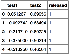
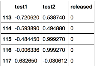
Save the training set and target class labels in separate NumPy arrays. Display the data. Red color corresponds to defective chips, green - normal.

 X = data.ix[:,:2].values y = data.ix[:,2].values 

 plt.scatter(X[y == 1, 0], X[y == 1, 1], c='green', label='') plt.scatter(X[y == 0, 0], X[y == 0, 1], c='red', label='') plt.xlabel(" 1") plt.ylabel(" 2") plt.title('2  ') plt.legend(); 

Define the function to display the classifier dividing curve

 def plot_boundary(clf, X, y, grid_step=.01, poly_featurizer=None): x_min, x_max = X[:, 0].min() - .1, X[:, 0].max() + .1 y_min, y_max = X[:, 1].min() - .1, X[:, 1].max() + .1 xx, yy = np.meshgrid(np.arange(x_min, x_max, grid_step), np.arange(y_min, y_max, grid_step)) #     [x_min, m_max]x[y_min, y_max] #      Z = clf.predict(poly_featurizer.transform(np.c_[xx.ravel(), yy.ravel()])) Z = Z.reshape(xx.shape) plt.contour(xx, yy, Z, cmap=plt.cm.Paired) 

Polynomial features to the extent $$$d$ for two variables $$$x_1$ and $$$x_2$ we call the following:

For example, for $$$d = 3$ these will be the following signs:

By drawing the Pythagorean triangle, you figure out how many of these signs there will be for $$$d = 4,5 ...$ and in general for any $$$d$ .
Simply put, there are a lot of such signs exponentially, and to build, say, for 100 signs polynomial degrees 10 can be costly (and moreover, it is not necessary).

Create a sklearn object that will add to the matrix $$$X$ polynomial features down to degree 7 and we will teach logistic regression with the regularization parameter $$$C = 10 ^ {- 2}$ . Draw a dividing border.
We will also check the share of correct answers of the classifier on the training set. We see that the regularization turned out to be too strong, and the model was “underused”. The share of correct answers of the classifier on the training sample was equal to 0.627.

 poly = PolynomialFeatures(degree=7) X_poly = poly.fit_transform(X) 

 C = 1e-2 logit = LogisticRegression(C=C, n_jobs=-1, random_state=17) logit.fit(X_poly, y) plot_boundary(logit, X, y, grid_step=.01, poly_featurizer=poly) plt.scatter(X[y == 1, 0], X[y == 1, 1], c='green', label='') plt.scatter(X[y == 0, 0], X[y == 0, 1], c='red', label='') plt.xlabel(" 1") plt.ylabel(" 2") plt.title('2  .   C=0.01') plt.legend(); print("      :", round(logit.score(X_poly, y), 3))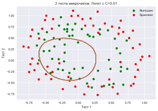 

Will increase $$$C$ to 1. Thus, we weaken the regularization, now in solving the weights of the logistic regression may be greater (in absolute value) than in the previous case. Now the share of correct classifier answers on the training set is 0.831.

 C = 1 logit = LogisticRegression(C=C, n_jobs=-1, random_state=17) logit.fit(X_poly, y) plot_boundary(logit, X, y, grid_step=.005, poly_featurizer=poly) plt.scatter(X[y == 1, 0], X[y == 1, 1], c='green', label='') plt.scatter(X[y == 0, 0], X[y == 0, 1], c='red', label='') plt.xlabel(" 1") plt.ylabel(" 2") plt.title('2  .   C=1') plt.legend(); print("      :", round(logit.score(X_poly, y), 3)) 

We will increase $$$C$ - up to 10 thousand. Now regularization is clearly not enough, and we are seeing retraining. You may notice that in the past case (when $$$C$ = 1 and "smooth" border) the proportion of correct answers of the model on the training sample is not much lower than in the 3 case, but on the new sample, one can imagine, the 2 model will work much better.
The share of the correct answers of the classifier on the training sample is 0.873.

 C = 1e4 logit = LogisticRegression(C=C, n_jobs=-1, random_state=17) logit.fit(X_poly, y) plot_boundary(logit, X, y, grid_step=.005, poly_featurizer=poly) plt.scatter(X[y == 1, 0], X[y == 1, 1], c='green', label='') plt.scatter(X[y == 0, 0], X[y == 0, 1], c='red', label='') plt.xlabel(" 1") plt.ylabel(" 2") plt.title('2  .   C=10k') plt.legend(); print("      :", round(logit.score(X_poly, y), 3))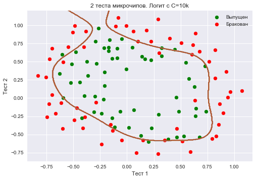 

To discuss the results, we rewrite the formula for the functional that is optimized in the logistic regression, in this form:

Where

• $$$\ mathcal {L}$ - logistic loss function summed over the entire sample
• $$$C$ - the inverse regularization coefficient (the same $$$C$ in the sklearn implementation of LogisticRegression)

Intermediate conclusions :

• the larger parameter $$$C$ , the more complex data dependencies can restore the model (intuitively $$$C$ Corresponds to the "complexity" of the model (model capacity))
• if the regularization is too strong (small values $$$C$ ), the solution to the problem of minimizing the logistic loss function may be when many weights are zeroed or become too small. They also say that the model is not “penalized” enough for errors (that is, in the functional $$$J$ "outweighs" the sum of the squares of the scales, and the error $$$\ mathcal {L}$ may be relatively large). In this case, the model will be under-trained (1 case)
• on the contrary, if the regularization is too weak (large values $$$C$ ), then the solution of the optimization problem can be a vector $$$w$ with large modulus components. In this case, a greater contribution to the optimized functionality. $$$J$ It has $$$\ mathcal {L}$ and, at ease, the model is too "afraid" to make a mistake on the objects of the training sample, therefore it will be retrained (case 3)
• what value $$$C$ choose, the logistic regression itself will not “understand” (or else they say “it will not learn”), that is, this cannot be determined by the solution of the optimization problem, which is the logistic regression (unlike weights $$$w$ ). In the same way, the decision tree cannot “self-understand” what constraint on depth to choose (in one learning process). therefore $$$C$ This is a hyperparameter of the model, which is configured for cross-validation, like max_depth for the tree.

Setting the regularization parameter

Now we find the optimal (in this example) value of the regularization parameter $$$C$ . This can be done with the help of LogisticRegressionCV - sorting parameters on the grid, followed by cross-validation. This class was created specifically for logistic regression (effective algorithms of parameter search are known for it), for an arbitrary model we would use GridSearchCV, RandomizedSearchCV or, for example, special optimization algorithms for hyperparameters implemented in hyperopt.

 skf = StratifiedKFold(n_splits=5, shuffle=True, random_state=17) c_values = np.logspace(-2, 3, 500) logit_searcher = LogisticRegressionCV(Cs=c_values, cv=skf, verbose=1, n_jobs=-1) logit_searcher.fit(X_poly, y) 

Let us see how the quality of the model (the proportion of correct answers in the training and validation samples) changes as the hyperparameter changes $$$C$ .

Select the section with the "best" values ​​of C.

As we remember, such curves are called validation , earlier we built them manually, but in sklearn for them their construction is special methods that we will also use now.

4. Where logistic regression is good and where not so

IMDB Movie Review Analysis

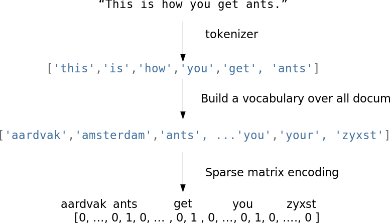
We will solve the problem of binary classification of IMDB movie reviews. There is an educational sample with marked reviews, according to 12,500 reviews it is known that they are good, even about 12,500 - that they are bad. It’s not so easy to start machine learning right away, because the finished matrix $$$X$ no - it must be cooked. We will use the simplest approach - a bag of words ("Bag of words"). With this approach, signs of the recall will be indicators of the presence of each word in it from the whole corpus, where the corpus is the set of all the responses. The idea is illustrated with a picture.

 from __future__ import division, print_function #    Anaconda import warnings warnings.filterwarnings('ignore') import numpy as np import matplotlib.pyplot as plt %matplotlib inline import seaborn as sns import numpy as np from sklearn.datasets import load_files from sklearn.feature_extraction.text import CountVectorizer, TfidfTransformer, TfidfVectorizer from sklearn.linear_model import LogisticRegression from sklearn.svm import LinearSVC 

 reviews_train = load_files("YOUR PATH") text_train, y_train = reviews_train.data, reviews_train.target 

 print("Number of documents in training data: %d" % len(text_train)) print(np.bincount(y_train)) 

 #     reviews_test = load_files("YOUR PATH") text_test, y_test = reviews_test.data, reviews_test.target print("Number of documents in test data: %d" % len(text_test)) print(np.bincount(y_test)) 

An example of a bad review:

'Words can \' t describe how bad this movie is. I can't explain it by writing only. Movie movie movie movie can you be. Not that I recommend you to do that. There are so many clich \ xc3 \ xa9s mistakes you can imagine. To start with the technical first. But don't mention the coloring of the plane. It was painted in the original Boeing livery. Very bad. The plot is stupid and has been done much more. I lost count of it really early. Also, I was on the bad guys \ 'side all the time in the movie, because the good guys were so stupid. "Executive Decision" should not be a choice over this one, even the "Turbulence" -movies are better. In fact, every other movie is better than this one. '

An example of a good review:

"Little plays your movie pretty well in this" little nice movie ". It’s a bit different. It shows us that we’re not getting any advantage. If you can get it \ xc2 \ xb4d be an investment! '

Simple word count

Create a dictionary of all words using CountVectorizer. A total of 74849 unique words in the sample. If you look at examples of the resulting "words" (better to call them tokens), you can see that we missed many important stages of text processing (automatic text processing - this could be the subject of a separate series of articles).

 cv = CountVectorizer() cv.fit(text_train) print(len(cv.vocabulary_)) #74849 

 print(cv.get_feature_names()[:50]) print(cv.get_feature_names()[50000:50050]) 

Encode sentences from the texts of the training sample with indices of incoming words. Use sparse format. Let's transform also test selection.

 X_train = cv.transform(text_train) X_test = cv.transform(text_test) 

Let's train a logistic regression and look at the shares of correct answers in the training and test samples. It turns out that on the test sample we correctly guess the tonality of approximately 86.7% of reviews.

 %%time logit = LogisticRegression(n_jobs=-1, random_state=7) logit.fit(X_train, y_train) print(round(logit.score(X_train, y_train), 3), round(logit.score(X_test, y_test), 3)) 

Model odds can be beautifully displayed.

 def visualize_coefficients(classifier, feature_names, n_top_features=25): # get coefficients with large absolute values coef = classifier.coef_.ravel() positive_coefficients = np.argsort(coef)[-n_top_features:] negative_coefficients = np.argsort(coef)[:n_top_features] interesting_coefficients = np.hstack([negative_coefficients, positive_coefficients]) # plot them plt.figure(figsize=(15, 5)) colors = ["red" if c < 0 else "blue" for c in coef[interesting_coefficients]] plt.bar(np.arange(2 * n_top_features), coef[interesting_coefficients], color=colors) feature_names = np.array(feature_names) plt.xticks(np.arange(1, 1 + 2 * n_top_features), feature_names[interesting_coefficients], rotation=60, ha="right"); 

 def plot_grid_scores(grid, param_name): plt.plot(grid.param_grid[param_name], grid.cv_results_['mean_train_score'], color='green', label='train') plt.plot(grid.param_grid[param_name], grid.cv_results_['mean_test_score'], color='red', label='test') plt.legend(); 

 visualize_coefficients(logit, cv.get_feature_names())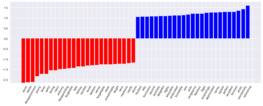 

We select the regularization coefficient for the logistic regression. We use sklearn.pipeline, since the CountVectorizer should be correctly applied only to the data on which the model is currently being trained (so as not to "peep" into the test sample and not count the word occurrence frequency on it). In this case, the pipeline sets the sequence of actions: apply the CountVectorizer, then train the logistic regression. So we raise the share of correct answers to 88.5% for cross-validation and 87.9% for deferred sampling.

 from sklearn.pipeline import make_pipeline text_pipe_logit = make_pipeline(CountVectorizer(), LogisticRegression(n_jobs=-1, random_state=7)) text_pipe_logit.fit(text_train, y_train) print(text_pipe_logit.score(text_test, y_test)) from sklearn.model_selection import GridSearchCV param_grid_logit = {'logisticregression__C': np.logspace(-5, 0, 6)} grid_logit = GridSearchCV(text_pipe_logit, param_grid_logit, cv=3, n_jobs=-1) grid_logit.fit(text_train, y_train) grid_logit.best_params_, grid_logit.best_score_ plot_grid_scores(grid_logit, 'logisticregression__C') grid_logit.score(text_test, y_test) 

Now the same, but with a random forest. We see that with the logistic regression we achieve a greater share of correct answers with less effort. The forest works longer, on a delayed sample of 85.5% correct answers.

 from sklearn.ensemble import RandomForestClassifier forest = RandomForestClassifier(n_estimators=200, n_jobs=-1, random_state=17) forest.fit(X_train, y_train) print(round(forest.score(X_test, y_test), 3)) 

XOR problem

Now consider an example where linear models do worse.

Linear classification methods still build a very simple dividing surface - the hyperplane. The most famous toy example, in which classes cannot be divided without errors by a hyperplane (that is, direct, if it is 2D), has been given the name "the XOR problem".

XOR is XOR, a Boolean function with the following truth table:

XOR gave the name to a simple binary classification problem, in which classes are represented by diagonal clouds and intersecting point clouds.

 #   rng = np.random.RandomState(0) X = rng.randn(200, 2) y = np.logical_xor(X[:, 0] > 0, X[:, 1] > 0) 

 plt.scatter(X[:, 0], X[:, 1], s=30, c=y, cmap=plt.cm.Paired); 

 def plot_boundary(clf, X, y, plot_title): xx, yy = np.meshgrid(np.linspace(-3, 3, 50), np.linspace(-3, 3, 50)) clf.fit(X, y) # plot the decision function for each datapoint on the grid Z = clf.predict_proba(np.vstack((xx.ravel(), yy.ravel())).T)[:, 1] Z = Z.reshape(xx.shape) image = plt.imshow(Z, interpolation='nearest', extent=(xx.min(), xx.max(), yy.min(), yy.max()), aspect='auto', origin='lower', cmap=plt.cm.PuOr_r) contours = plt.contour(xx, yy, Z, levels=[0], linewidths=2, linetypes='--') plt.scatter(X[:, 0], X[:, 1], s=30, c=y, cmap=plt.cm.Paired) plt.xticks(()) plt.yticks(()) plt.xlabel(r'$<!-- math>$inline$x_1$inline$</math -->$') plt.ylabel(r'$<!-- math>$inline$x_2$inline$</math -->$') plt.axis([-3, 3, -3, 3]) plt.colorbar(image) plt.title(plot_title, fontsize=12); 

 plot_boundary(LogisticRegression(), X, y, "Logistic Regression, XOR problem") 

 from sklearn.preprocessing import PolynomialFeatures from sklearn.pipeline import Pipeline 

 logit_pipe = Pipeline([('poly', PolynomialFeatures(degree=2)), ('logit', LogisticRegression())]) 

 plot_boundary(logit_pipe, X, y, "Logistic Regression + quadratic features. XOR problem") 

Obviously, it is impossible to draw a straight line in such a way that without errors one class can be separated from another. Therefore, logistic regression is not good at this task.

But if you submit to the input polynomial signs, in this case up to 2 degrees, the problem is solved.

Here, the logistic regression still built a hyperplane, but in a 6-dimensional feature space $$$1, x_1, x_2, x_1 ^ 2, x_1x_2$ and $$$x_2 ^ 2$ . In projection on the original feature space $$$x_1, x_2$ the border is non-linear.

In practice, polynomial features really help, but building them explicitly is computationally inefficient. SVM works much faster with a sound stunt. With this approach, only the distance between objects (defined by the kernel function) is considered in a space of high dimensionality, and obviously there is no need to produce a combinatorially large number of features. You can read about this in detail in the course of Evgeny Sokolov (mathematics is already serious).

5. Validation and learning curves

We have already gained insight into model validation, cross-validation, and regularization.
Now consider the main question:

If the quality of the model does not suit us, what to do?

• Make the model harder or easier?
• Add more signs?
• Or do we just need more data for training?

Answers to these questions do not always lie on the surface. In particular, sometimes the use of a more complex model will lead to a deterioration in performance. Or the addition of observations will not lead to tangible changes. The ability to make the right decision and choose the right way to improve the model, strictly speaking, distinguishes a good specialist from a bad one.

We will work with familiar data on the outflow of customers of the telecom operator.

 from __future__ import division, print_function #    Anaconda import warnings warnings.filterwarnings('ignore') %matplotlib inline from matplotlib import pyplot as plt import seaborn as sns import numpy as np import pandas as pd from sklearn.preprocessing import PolynomialFeatures from sklearn.pipeline import Pipeline from sklearn.preprocessing import StandardScaler from sklearn.linear_model import LogisticRegression, LogisticRegressionCV, SGDClassifier from sklearn.model_selection import validation_curve data = pd.read_csv('../../data/telecom_churn.csv').drop('State', axis=1) data['International plan'] = data['International plan'].map({'Yes': 1, 'No': 0}) data['Voice mail plan'] = data['Voice mail plan'].map({'Yes': 1, 'No': 0}) y = data['Churn'].astype('int').values X = data.drop('Churn', axis=1).values 

We will teach the logistic regression with a stochastic gradient descent. For now, we will explain this by saying that this is faster, but later in the program we have a separate article about this matter. We construct validation curves showing how the quality (ROC AUC) on the training and verification sample varies with the change of the regularization parameter.

 alphas = np.logspace(-2, 0, 20) sgd_logit = SGDClassifier(loss='log', n_jobs=-1, random_state=17) logit_pipe = Pipeline([('scaler', StandardScaler()), ('poly', PolynomialFeatures(degree=2)), ('sgd_logit', sgd_logit)]) val_train, val_test = validation_curve(logit_pipe, X, y, 'sgd_logit__alpha', alphas, cv=5, scoring='roc_auc') def plot_with_err(x, data, **kwargs): mu, std = data.mean(1), data.std(1) lines = plt.plot(x, mu, '-', **kwargs) plt.fill_between(x, mu - std, mu + std, edgecolor='none', facecolor=lines[0].get_color(), alpha=0.2) plot_with_err(alphas, val_train, label='training scores') plot_with_err(alphas, val_test, label='validation scores') plt.xlabel(r'$\alpha$'); plt.ylabel('ROC AUC') plt.legend();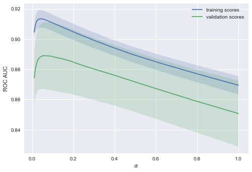 

The trend is visible immediately, and it is very common.

• For simple models, training and validation errors are somewhere nearby, and they are great. This suggests that the model was under - educated : that is, it does not have a sufficient number of parameters.

  
  

• For highly sophisticated models, training and validation errors are significantly different. This can be explained by overtraining : when there are too many parameters or there is a lack of regularization, the algorithm can be "distracted" by the noise in the data and lose the main trend.

  
  

How much data is needed?

It is known that the more data a model uses, the better. But as we understand in a particular situation, will the new data help? Say, is it advisable for us to spend N \ $ on assessors to double the sample?

Since there may not yet be new data, it is reasonable to vary the size of the available training sample and see how the quality of the solution of the problem depends on the amount of data on which we trained the model. This is how learning curves are obtained.

The idea is simple: we display an error as a function of the number of examples used for training. In this case, the parameters of the model are fixed in advance.

Let's see what we get for the linear model. We set the regularization coefficient large.

 from sklearn.model_selection import learning_curve def plot_learning_curve(degree=2, alpha=0.01): train_sizes = np.linspace(0.05, 1, 20) logit_pipe = Pipeline([('scaler', StandardScaler()), ('poly', PolynomialFeatures(degree=degree)), ('sgd_logit', SGDClassifier(n_jobs=-1, random_state=17, alpha=alpha))]) N_train, val_train, val_test = learning_curve(logit_pipe, X, y, train_sizes=train_sizes, cv=5, scoring='roc_auc') plot_with_err(N_train, val_train, label='training scores') plot_with_err(N_train, val_test, label='validation scores') plt.xlabel('Training Set Size'); plt.ylabel('AUC') plt.legend() plot_learning_curve(degree=2, alpha=10)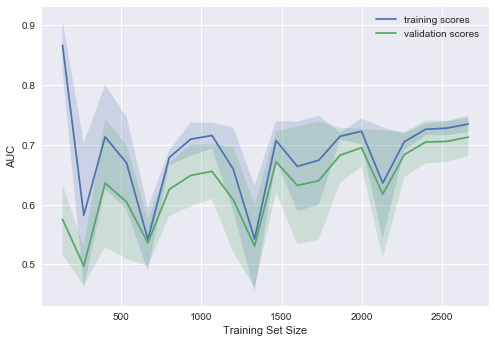 

: - , . , "", .

, , , .

, "", . , – . , 10 . , . " – 10 " .

, ( 0.05)?

– , ( ), .

( $$$alpha=10^{-4}$ )?

– AUC , .

, , , .

• - , ( ),
• , :
• , , —
• , —
• — , :
• , –
• , .

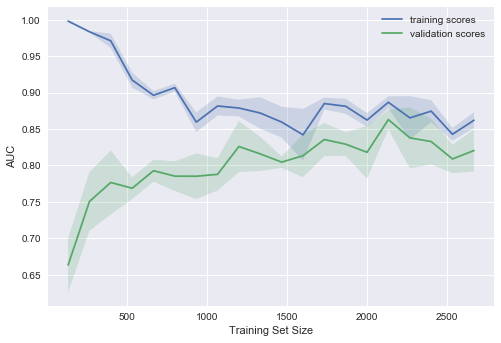
6.

Pros:

• ,
• , ( ), ( )
• ( ) – , – $$$\exp^{\beta_i}$ $$$x_i$ 1 .,
• ( , , )
• ,

Minuses:

• , ,
• - , , , , SVM ( /)

7. № 4

, .

: , TfidfVectorize r DictVectorizer , Ridge . - ( ).

8.

• – Jupyter notebooks
• : ,
• , , "Deep Learning" (I. Goodfellow, Y. Bengio, A. Courville, 2016);
• – rushter . ;
• ( GitHub). , ;
• GitHub (.). .

mephistopheies ( ). – . (- 2017)– aiho ( ) das19 ( ). bauchgefuehl ( ) .