LIFT: Learned Invariant Feature Transform

Introduction

In recent years, ubiquitous neural networks are finding more and more applications in various fields of knowledge, crowding out the classical algorithms used for many years. The area of computer vision, where year after year more and more problems are solved with the help of modern neural networks, is no exception. It is time to write about another traditional fighter in the war, "Traditional Vision vs. Deep Training." For many years, the SIFT (Scale-invariant Feature Transform) algorithm, proposed back in 1999, reigned supreme in the task of finding local features of images (the so-called key points), many folded their heads in trying to surpass it, but only Deep Learning succeeded. So, meet, a new algorithm for finding local features - LIFT (Learned Invariant Feature Transform).

Need for Data

For deep learning to work, you need a lot of data, otherwise the magic will not work. And we need not all kinds of data, but those that would be a representative representation of the task that we want to solve. So, let's look at what man-made detectors / descriptors of special points can do:

Invariance to the location in the picture.
Invariance to the angle of rotation.
Invariance to scale.

Okay, so we need a dataset containing a bunch of points where for each particular point there will be a lot of samples obtained from different angles. You can, of course, take arbitrary images, cut points from them, and then use synthetically generated affine transformations to get datasets of arbitrarily large size. But synthetics are bad because there are always some limitations on the accuracy of modeling.
real cases. Real data sets that meet our requirements arise when solving some applied problems of computer vision. For example, when 3D reconstructing scenes shot from multiple angles, we do something like the following:

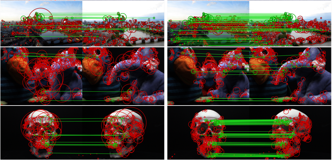
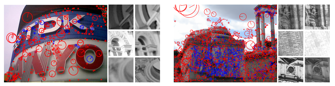
For each image of the scene we find special points.
We find correspondences between special points from different images.
But based on this information, we calculate the spatial arrangement of each frame (parameterized through $[R, t]$ those. rotation and translation relative to the origin).
Using the triangulation procedure, we find the 3D positions of all singular points.
Using the spreading optimization aki Bundle Adjustment (most often the algorithm, derived from the Levenberg-Marquardt method), we obtain more accurate information about the location of points in space.
Any different postprocessing. For example, you can stretch a polygonal model on a cloud of points to get smooth surfaces.

As a by-product of the operation of such an algorithm, we get a cloud of points, where each 3D point corresponds to several of its 2D positions (projections) on the scene frames. Here is a cloud - this is exactly the dataset we need. Without taking much interest in the intricacies of Structure From Motion, the authors took a couple of publicly available datasets for 3D reconstruction, drove them through a publicly available tool for building a cloud of points (VisualSFM), and then used the resulting data set in their experiments. As stated, the mesh trained on such a set is also generalized to other types of scenes.

Grids, nets, nets

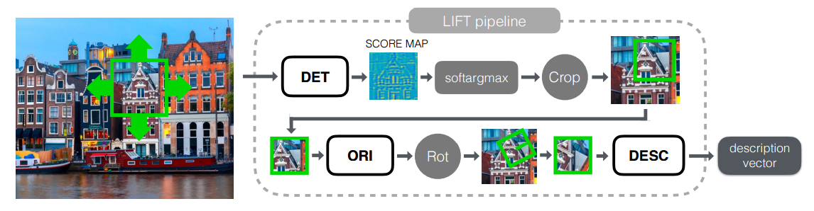
We have dealt with dataset, so it's time to move on to the most interesting, namely, the study of grids. The whole grid can be divided into 3 logical blocks:

Detector - is responsible for finding special points on the entire image as a whole.
Rotation Estimator - determines the orientation of the point and turns the patch around it so that the rotation angle is equal to zero.
Descriptor - takes as input a patch, by which it builds a unique (here how it will turn out) vector describing this patch. These vectors can already be used, for example, in order to calculate the Euclidean distance between a pair of points and understand whether they are similar or not.

First, we consider the inference for this model as a whole, and then all the blocks separately and exactly how they train.

Inference

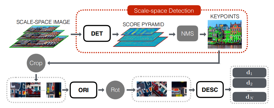
The search for special points and the calculation of their descriptors occurs in several stages:

To begin with, we build a pyramid of images (i.e., we bring the original image to several scales to obtain scale-invariant features) for the original image.
Each layer of the pyramid is run through the network-detector and the Score Map pyramid is calculated.
Using the Non-Maximum Suppression procedure, we find the strongest candidates for particular points.
For each singular point, cut a patch that includes the singular point and some of its neighborhoods.
Align the orientation of each patch with the Orientation Estimator.
We calculate the handle for each aligned patch.
We use the obtained descriptors for the standard feature matching procedure.

Descriptor

Since the time of the SIFT feature, it is known that even if we are not very good at finding truly unique points, but we can build a cool descriptor for each of them, then we can most likely solve the problem. Therefore, we will begin the review from the end, namely with the construction of a descriptor for the singular point already found. Generally speaking, any convolutional mesh, taking a picture (patch) as input, yields some description of this picture, which can already be used as a descriptor. But, as practice shows, there is no need to take a huge network, such as, for example, VGG16, ResNet-152, Inception etc., a small network is enough for us: 2-3 convolutional layers with activations in the form of hyperbolic tangents
and other small things like batch normalization, etc.

For definiteness, let's denote our network descriptor. $d = h_ {p} (p _ {\ theta})$ where $h (...)$ - descriptor convolution network, $p$ - its parameters $p _ {\ theta}$ - Patch with zero angle (obtained from the Rotation Estimator).

For each singular point we make two pairs:

$(p _ {\ theta} ^ {1}, p _ {\ theta} ^ 2)$ - a pair of patches corresponding to the projections of the same particular point.
$(p _ {\ theta} ^ {1}, p _ {\ theta} ^ 3)$ - a couple of patches where the first one belongs to a particular point and the second (negative sample) does not. At the same time, the “negative” patch is selected from a certain neighborhood, not too far from positive. In the process of training the neighborhood decreases, so that negative samples become more and more difficult.

In the process of learning we will minimize the loss-function of the following form:

L_{d e s c} (p_{t h e t a}^{k}, p_{t h e t a}^{l}) = b e g i n c a s e s | h_{p} (p_{t h e t a}^{k}) - h_{p} (p_{t h e t a}^{l}) |_{2}, f o r p o s i t i v e s m a x (0, C - | h_{p} (p_{t h e t a}^{k}) - h_{p} (p_{t h e t a}^{l}) |_{2}), f o r n e g a t i v e s e n d c a s e s

$L_ {desc} (p _ {\ theta} ^ k, p _ {\ theta} ^ l) = \ begin {cases} \ | h_p (p _ {\ theta} ^ k) - h_p (p _ {\ theta} ^ l ) \ | _ {2}, for \ positives \\ max (0, C - \ | h_p (p _ {\ theta} ^ k) - h_p (p _ {\ theta} ^ l) \ | _ {2}), for \ negatives \ end {cases}$

Those. in essence, we want the Euclidean distance between similar points to be small, and between points that are not similar to each other to be far away.

Rotation estimator

Since we can observe the same point not only from different points of space, but also from different angles of inclination, we must be able to build the same descriptor for the same particular point, no matter from what angle we observe it. But instead of teaching Descriptor to memorize all possible angles of inclination for the same point, it is proposed to use an intermediate computational block that will determine the orientation of the patch in space (Rotation Estimator) and “turn” the patch to some state invariant to rotation (Spatial Transform). Of course, it would be possible to use the block for calculating the orientation of the patch in space, taken from the algorithm for constructing SIFT features, but outside the 21st century it is now accepted to reduce any computer vision problem to machine learning. So we will use another convolutional neural network to solve this problem.

So, we denote our neural network as: $\ theta = g _ {\ phi} (p)$ where $\ phi$ - network settings, and $p$ - source patch.

Let's take a couple of patches as a sample. $P ^ 1$ , $P ^ 2$ belonging to one singular point, but having different angles of inclination, as well as their spatial coordinates $x ^ 1$ , $x ^ 2$ .

In the process of learning we will minimize the following loss-function:

L_{o r i e n t a t i o n} (P^{1}, x^{1}, P^{2}, x^{2}) = | h_{p} (G (P^{1}, x^{1})) - h_{p} (G (P^{2}, x^{2})) |_{2}

$L_ {orientation} (P ^ 1, x ^ 1, P ^ 2, x ^ 2) = \ | h_p (G (P ^ 1, x ^ 1)) - h_p (G (P ^ 2, x ^ 2)) \ | _2$

Where $G (P, x)$ - patch obtained after the procedure for correcting its orientation, $G (P, x) = Rot (P, x, g _ {\ phi} (Crop (P, x)))$ .

Those. when training a network, we turn patches, with different angles of inclination, so that the Euclidean distance between their descriptors becomes minimal.

Detector

It remains to consider the last step, namely the direct detection of specific points on the original image. The essence of this network is that the entire image is driven through it, and some feature map is expected at the output, for which special points on the source image correspond to strong responses.

In spite of the fact that when the model is inference, the detector is triggered on the entire image at once, in the course of the training we will chase it only for individual patches.

The calculation of the detector consists of two steps: first we must calculate the Score Map for the patch, which will then determine the position of the singular point:

S = f_{m u} (P) = s u m_{n}^{N} b e t a_{n} m a x_{m}^{M} (W_{m n} * P + b_{m n})

$S = f _ {\ mu} (P) = \ sum_n ^ N \ beta_n \ max_m ^ M (W_ {mn} * P + b_ {mn})$

and then, calculate the position of the singular point:

x = s o f t a r g m a x (S)

$x = softargmax (S)$

Where $softargmax$ Is a function that calculates a weighted center of mass with weights that are the result of a calculation $softmax$ :

softargmax (S) = \ frac {\ sum_ {y} \ exp (\ beta S (y)) y} {\ sum_ {y} \ exp (\ beta S (y))

$softargmax (S) = \ frac {\ sum_ {y} \ exp (\ beta S (y)) y} {\ sum_ {y} \ exp (\ beta S (y))$

where y is the position within Score Map, $\ beta$ - hyperparameter responsible for the coefficient of "blurring" softmax-function.

When training the detector, we will take four patches. $(P ^ 1, P ^ 2, P ^ 3, P ^ 4)$ where $P ^ 1, P ^ 2$ - projections of the same singular point, $P ^ 3$ - projection of another singular point, $P ^ 4$ - A patch not belonging to a particular point. For the collection of such patches we will minimize the following loss-function:

L_{d e t e c t o r} (P^{1}, P^{2}, P^{3}, P^{4}) = g a m m a L_{c l a s s} (P^{1}, P^{2}, P^{3}, P^{4}) + L_{p a i r} (P^{1}, P^{2})

$L_ {detector} (P ^ 1, P ^ 2, P ^ 3, P ^ 4) = \ gamma L_ {class} (P ^ 1, P ^ 2, P ^ 3, P ^ 4) + L_ {pair } (P ^ 1, P ^ 2)$

Where $\ gamma$ - balancing parameter for two members of the loss function.
Member of the loss, responsible for the correct classification of positives and negatives:

L_{c l a s s} (P^{1}, P^{2}, P^{3}, P^{4}) = s u m_{i = 1}^{4} a l p h a_{i} m a x (0, 1 - s o f t m a x (f_{m u} (P^{i})) y_{i})^{2}

$L_ {class} (P ^ 1, P ^ 2, P ^ 3, P ^ 4) = \ sum_ {i = 1} ^ {4} \ alpha_i max (0, 1 - softmax (f _ {\ mu} ( P ^ i)) y_i) ^ 2$

Loss member, responsible for the exact localization of singular points:

L_{p a i r} (P^{1}, P^{2}) = | h_{p} (G (P^{1}, s o f t a r g m a x (f_{m u} (P^{1})))) - h_{p} (G (P^{2}, s o f t a r g m a x (f_{m u} (P^{2})))) |_{2}

$L_ {pair} (P ^ 1, P ^ 2) = \ | h_p (G (P ^ 1, softargmax (f _ {\ mu} (P ^ 1)))) - h_p (G (P ^ 2, softargmax (f _ {\ mu} (P ^ 2)))) \ | _2$

Training

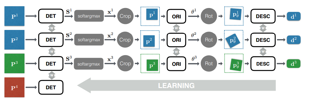
The whole network trains in the fashionable fashion now End-To-End, i.e. Immediately learn all parts of the network in parallel as Siamese networks. At the same time, for each of the 4 used in training, the patches create a separate network brunch with sharring weights between them.

Experiments

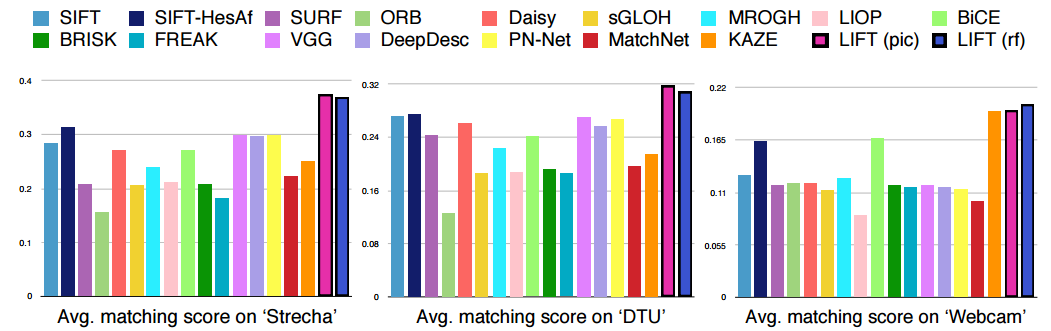
Comparing with the existing methods for finding particular points, the authors concluded that their approach is state of the art.

And the results of their network can be viewed in the following video:

Conclusion

The presented work is another confirmation of the fact that the time of traditional methods of computer vision is taking place, and it is being replaced by the era of Sainz. And once again coming up with an ingenious heuristics, solving some complex problem, you should think: is it possible to formulate a task so that the computer could independently iterate over millions of heuristics and choose the one that solves the problem in the best way.