Electrical circuit simulation

This publication provides instructions for modeling an electrical circuit using the state variable method.

This publication is in order to be in Russian at least one how2 on the simulation of electrical circuits by this method. At one time I googled a lot and never once did I come across normal material. All the manuals and textbooks contained only theory. In addition, none of the materials I found contained a complete solution cycle:

scheme ⟶ equations ⟶ numerical solution ⟶ graphics.

Actually, this is the algorithm of actions.
')
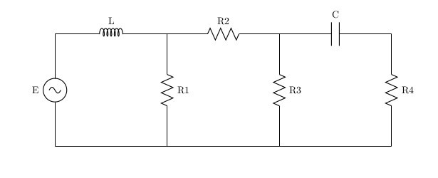
The scheme is, now you need to make equations using the laws of Ohm and Kirchhoff.

Component equations:

C * f r a c d U_{c} d t = i_{c}; L * f r a c d i_{l} d t = U_{L};

$C * \ frac {d {U_ {c}}} {d {t}} = i_ {c}; L * \ frac {d {i_ {l}}} {d {t}} = U_ {L};$

U_{1} = i_{1} * R_{1}; U_{2} = i_{2} * R_{2}; U_{3} = i_{3} * R_{3}; U_{4} = i_{4} * R_{4}; U_{1} = i_{1} * R_{1};

$U_ {1} = i_ {1} * R_ {1}; U_ {2} = i_ {2} * R_ {2}; U_ {3} = i_ {3} * R_ {3}; U_ {4} = i_ {4} * R_ {4}; U_ {1} = i_ {1} * R_ {1};$

Contour equations:

E - U_{L} - U_{1} = 0;

$E-U_ {L} -U_ {1} = 0;$

U_{1} - U_{2} - U_{3} = 0;

$U_ {1} -U_ {2} -U_ {3} = 0;$

U_{3} - U_{C} - U_{4} = 0;

$U_ {3} -U_ {C} -U_ {4} = 0;$

Nodal equations:

i_{L} - i_{1} - i_{2} = 0;

$i_ {L} - i_ {1} - i_ {2} = 0;$

i_{2} - i_{3} - i_{4} = 0;

$i_ {2} - i_ {3} - i_ {4} = 0;$

i_{c} = i_{4};

$i_ {c} = i_ {4};$

Now we need to derive differential equations. I note that in this method, it is customary to take charge of capacitors and flux couplings of inductances as state variables. Knowing these values, it is possible to derive any voltages and currents of nodes and branches. Also:

Equations must be independent;
The equations should include only state and source variables; all other variables must be expressed through state variables;
The first derivative of the state variables must enter the left side of each equation; on the right side there should be no derivatives.

We derive the first differential equation:

U_{L} = E - U_{1} = E - U_{2} - U_{3} = E - U_{2} - U_{C} - U_{4};

$U_ {L} = E-U_ {1} = E-U_ {2} -U_ {3} = E-U_ {2} -U_ {C} -U_ {4};$

U_{L} = E - i_{2} * R_{2} - U_{C} - i_{C} * R_{4} = E - (i_{L} - f r a c E - U_{L} R_{1}) * R_{2} - U_{C} - i_{C} * R_{4};

$U_ {L} = E-i_ {2} * R_ {2} -U_ {C} -i_ {C} * R_ {4} = E- (i_ {L} - \ frac {E-U_ {L} } {R_ {1}}) * R_ {2} -U_ {C} -i_ {C} * R_ {4};$

U_{L} = E - i_{L} * R_{2} + E * f r a c R_{2} R_{1} - U_{L} * f r a c R_{2} R_{1} - U_{C} - i_{C} * R_{4};

$U_ {L} = E-i_ {L} * R_ {2} + E * \ frac {R_ {2}} {R_ {1}} - U_ {L} * \ frac {R_ {2}} {R_ {1}} - U_ {C} -i_ {C} * R_ {4};$

U_{L} * f r a c R_{1} + R_{2} R_{1} = E * f r a c R_{1} + R_{2} R_{1} - i_{L} * R_{2} - U_{C} - i_{C} * R_{4};

$U_ {L} * \ frac {R_ {1} + R_ {2}} {R_ {1}} = E * \ frac {R_ {1} + R_ {2}} {R_ {1}} - i_ { L} * R_ {2} -U_ {C} -i_ {C} * R_ {4};$

i_{C} = i_{L} - i_{1} - i_{3} = i_{L} - f r a c E - U_{L} R_{1} - f r a c U_{C} + i_{C} * R_{4} R_{3};

$i_ {C} = i_ {L} -i_ {1} -i_ {3} = i_ {L} - \ frac {E-U_ {L}} {R_ {1}} - \ frac {U_ {C} + i_ {C} * R_ {4}} {R_ {3}};$

i_{C} f r a c R_{3} + R_{4} R_{3} = i_{L} - f r a c E - U_{L} R_{1} - f r a c U_{C} R_{3};

$i_ {C} \ frac {R_ {3} + R_ {4}} {R_ {3}} = i_ {L} - \ frac {E-U_ {L}} {R_ {1}} - \ frac { U_ {C}} {R_ {3}};$

Substitute the capacitor current into the coil voltage equation:

U_{L} * f r a c R_{1} + R_{2} R_{1} = E * f r a c R_{1} + R_{2} R_{1} - i_{L} * R_{2} - U_{C} - f r a c R_{3} * R_{4} R_{3} + R 4 * (i_{L} - f r a c E R_{1} + f r a c U_{L} R_{1} - f r a c U_{C} R_{3});

$U_ {L} * \ frac {R_ {1} + R_ {2}} {R_ {1}} = E * \ frac {R_ {1} + R_ {2}} {R_ {1}} - i_ { L} * R_ {2} -U_ {C} - \ frac {R_ {3} * R_ {4}} {R_ {3} + R {4}} * (i_ {L} - \ frac {E} { R_ {1}} + \ frac {U_ {L}} {R_ {1}} - \ frac {U_ {C}} {R_ {3}});$

Transforming the equation, we get the first differential equation:

L * f r a c d i_{L} d t = U_{L} = E - f r a c R_{1} (R_{1} + R_{2}) * (R_{3} + R_{4}) + R_{3} * R_{4} * (i_{L} * (R_{2} * (R_{3} + R_{4}) + R_{3}) - U_{C} * R_{3});

$L * \ frac {di_ {L}} {dt} = U_ {L} = E- \ frac {R_ {1}} {(R_ {1} + R_ {2}) * (R_ {3} + R_ {4}) + R_ {3} * R_ {4}} * (i_ {L} * (R_ {2} * (R_ {3} + R_ {4}) + R_ {3}) - U_ {C} * R_ {3});$

We derive the second differential equation:

i_{C} = i_{L} - i_{1} - i_{3} = i_{L} - f r a c E - U_{L} R_{1} - f r a c U_{C} R_{3} - f r a c i_{C} * R_{4} R_{3};

$i_ {C} = i_ {L} -i_ {1} -i_ {3} = i_ {L} - \ frac {E-U_ {L}} {R_ {1}} - \ frac {U_ {C} } {R_ {3}} - \ frac {i_ {C} * R_ {4}} {R_ {3}};$

C * f r a c d U_{c} d t = i_{c} = f r a c R_{3} C * (R_{3} + R_{4}) * (i_{L} - f r a c E - U_{L} R_{1} - f r a c U_{C} R_{3});

$C * \ frac {d {U_ {c}}} {d {t}} = i_ {c} = \ frac {R_ {3}} {C * (R_ {3} + R_ {4})} * (i_ {L} - \ frac {E-U_ {L}} {R_ {1}} - \ frac {U_ {C}} {R_ {3}});$

Now we have a system of differential equations that can be solved numerically:

b e g i n c a s e s L * f r a c d i_{L} d t = E - f r a c R_{1} (R_{1} + R_{2}) * (R_{3} + R_{4}) + R_{3} * R_{4} * (i_{L} * (R_{2} * (R_{3} + R_{4}) + R_{3}) - U_{C} * R_{3}); C * f r a c d U_{c} d t = f r a c R_{3} C * (R_{3} + R_{4}) * (i_{L} - f r a c E - U_{L} R_{1} - f r a c U_{C} R_{3}); e n d c a s e s

$\ begin {cases} L * \ frac {di_ {L}} {dt} = E- \ frac {R_ {1}} {(R_ {1} + R_ {2}) * (R_ {3} + R_ {4}) + R_ {3} * R_ {4}} * (i_ {L} * (R_ {2} * (R_ {3} + R_ {4}) + R_ {3}) - U_ {C} * R_ {3}); \\ C * \ frac {d {U_ {c}}} {d {t}} = \ frac {R_ {3}} {C * (R_ {3} + R_ {4})} * (i_ {L } - \ frac {E-U_ {L}} {R_ {1}} - \ frac {U_ {C}} {R_ {3}}); \ end {cases}$

We use the Euler method ~~because~~ ~~it's the easiest~~ and use Python:

X_{i} = X_{i - 1} + h * f r a c d X_{i - 1} d t

$X_ {i} = X_ {i-1} + h * \ frac {d {X_ {i-1}}} {d {t}}$

Program

import numpy as np import matplotlib.pyplot as plt #Input voltage amplitude AMP = 21.0 #Active components r1 = 2000.0; r2 = 10.0; r3 = 10.0; r4 =2000.0; #Reactive components c=0.0001; l=0.06; #Time components T=0.01; t0=0.0; step=T/1000; tf=T*10 steps=int(tf/step); #Input voltage def E(t): n=int(t/T) if ((t >= n*T )and(t <= n*T + T/2)): return AMP else: return 0.0 time = np.arange(t0, tf, step) ul = []; il = []; uc = []; ic = []; y = []; for i in range(0, steps, 1): y.append(E(time[i])) def dIl_dt(t): return float((1.0/l)*(E(t) - (r1/((r1+r2)*(r3+r4)+r3*r4) * (il[int(t/step)]*(r2*(r3+r4)+r3) - uc[int(t/step)]*r3)))) def dUc_dt(t): return float((1.0/c)* (r3/(r3+r4)) * (il[int(t/step)]-(E(t)-ul[int(t/step)])/r1 - uc[int(t/step)]/r3)) #Start condition ul.append(E(0)); il.append(0.0); uc.append(0.0); ic.append(0.0); #Euler method for i in range(1, steps, 1): il.append(il[i-1] + step*dIl_dt(time[i-1])) uc.append(uc[i-1] + step*dUc_dt(time[i-1])) ul.append(l*dIl_dt(time[i])) ic.append(c*dUc_dt(time[i])) plt.figure("charts") e = plt.subplot(311) e.plot(time, y) e.set_xlabel('time (s)') e.set_ylabel('E(t), (V)', color='b') plt.grid(True) UL = plt.subplot(312) UL.plot(time, ul) UL.set_xlabel('time (s)') UL.set_ylabel('Ul(t), (V)', color = 'b') IL = UL.twinx() IL.plot(time, il, 'r') IL.set_ylabel('Il(t), (A)', color = 'r') plt.grid(True) UC = plt.subplot(313) UC.plot(time, uc) UC.set_xlabel('time (s)') UC.set_ylabel('Uc(t), (V)', color = 'b') IC = UC.twinx() IC.plot(time, ic, color = 'r') IC.set_ylabel('Ic(t), (A)', color = 'r') plt.grid(True) plt.show()

Simulation results:

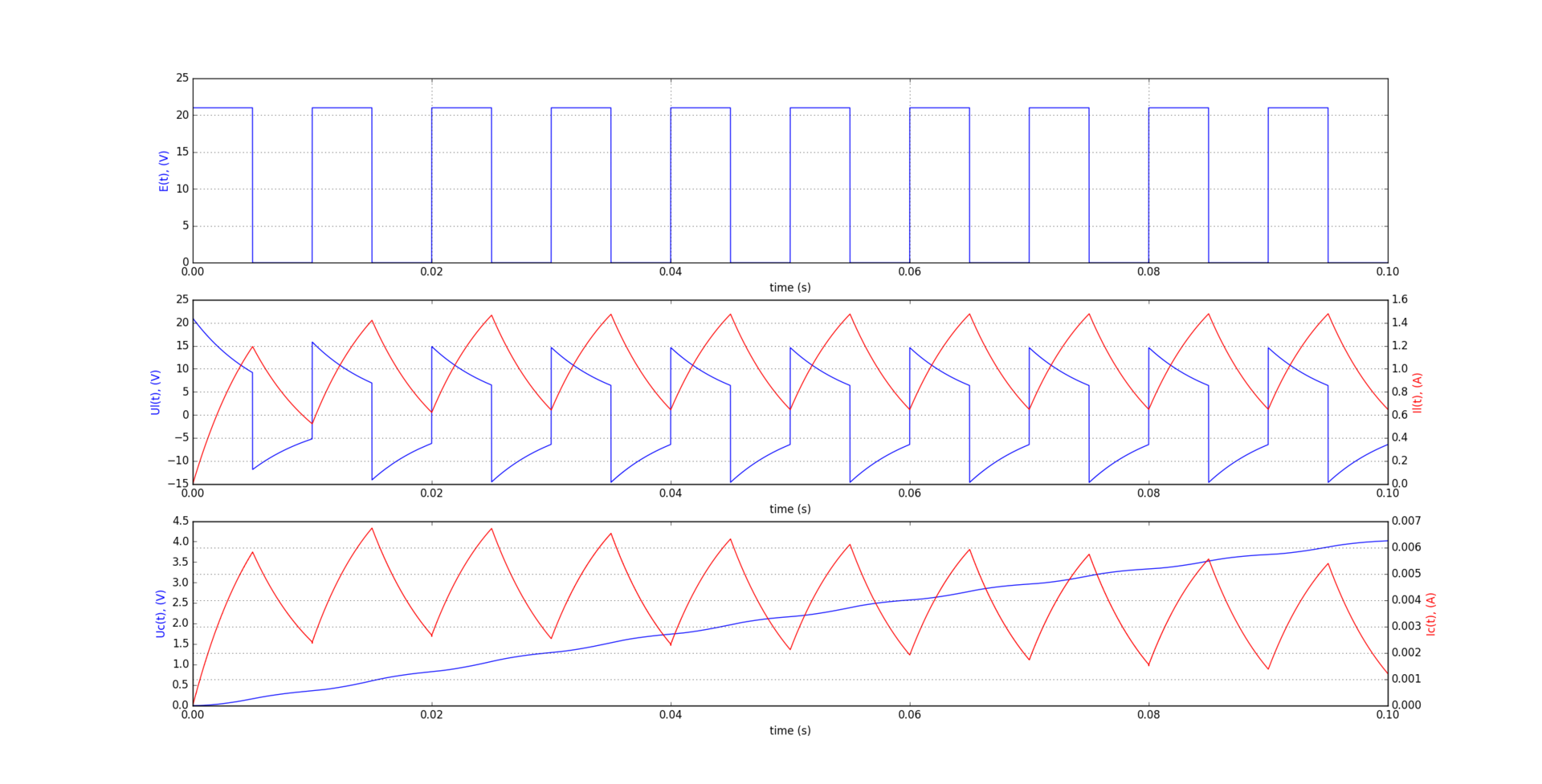
It is better to use other methods for solving difur for real calculations, and for obtaining graphs of voltages and currents of elements for self-learning, the simplest Euler method is sufficient. In electronics, the most common Newton-Raphson method is in most CAD systems it is this method that is used.

From the literature I advise books of PN Matkhanov. and Zebeke G.V.
And the manuals of all polytechnics (MSTU, St. Petersburg, Tomsk, etc.) and similar material are easier to throw out than to understand what is written there. Here is a catch phrase: “simplify is difficult, complicate is easy”.

Source: https://habr.com/ru/post/323590/

All Articles

Electrical circuit simulation

More articles: