Learning to learn. Create self-improving AI

Learning to learn

This time I conducted experiments on the topic of learning to learn, that is, algorithms that can learn how best to learn.

Objectives of the experiment:

1) Create an optimization algorithm that can be adapted in any standard way to any optimization problem or a set of problems. By the word "adapt" I mean "to make the algorithm very well cope with this task."
2) Adjust the algorithm for one task and see how its efficiency has changed in other tasks.

Why are optimization algorithms important at all?

Because so many tasks can be reduced to optimization problems. For example, in this article you can see how to reduce the task of driving a vehicle to an optimization problem.
In the example, we will test the algorithm on more traditional optimization problems, since this test will take less time than learning the neural network.

Task list

Our algorithm will have the following tasks:
')
1) The problem of polynomial regression. Given a certain function, it is necessary to construct a curve that will approximate the graph of this function by a graph of a 7th degree polynomial. The optimizer selects regression coefficients. The quality metric in this task is equal to the average deviation between the actual graph and the approximation. The function has many local optima, but it is smooth.
2) The problem on the quadratic function. The quality metric q = (k1-10) ^ 2 + (k2 + 15) ^ 2 + (k3 + 10 * k4-0.06) ^ 2 + ..., that is, it is equal to the sum of squares of certain linear functions of the coefficients that the optimizer selects . The function has many minima, but it is smooth.
3) The problem on a discrete function. The quality metric is calculated using the following algorithm: q = 1; if (k1> -2) {q + = 3}; if (k1 <0.2) {q + = 15}; ..., then the graph of the function of any variable will look like a certain step line. The function has few local optima, but it is not smooth.

As a training task, I will apply task 2 (to a quadratic function), the other two as test ones.

Optimizer

As an optimizing algorithm, I will use my own hand-written ensemble of algorithms, which I called Abatur. This ensemble includes several variants of coordinate descent, gradient descent, evolution, algorithm of a bee swarm. And the control algorithm, which with different probability causes different modules.

This is the main block of decision making in Abatura.

for i=1:sz(2) %optimizerData.optimizers -    reputation(i)=optimizerData.optimizers{i}.reputation; %optimizerData.optimizers{i}.reputation -    ,      reputationR(i)=reputation(i)*(1+0.5*randD()); end; [ampl,arg]=max(reputationR); [newK,dt]=feval(optimizerData.optimizers{arg}.name,optimizerData); optimizerData.dt=optimizerData.dt+dt; valNew=feval(optimizerData.func,newK); if(valNew>=valOld) optimizerData.kArr=newK; valOld=valNew; end; 

optimizerData.k is an array of Abatura parameters. As can be seen in the code above, these parameters determine everything: the steps of the gradient descent, the size of the populations, the likelihood of an optimizer to work.

Abatur himself cannot change these parameters, but some other algorithm that is engaged in Abatura optimization can change them. Abatura training consists in selecting parameters k that maximize its metric.

Quality metric learning to learn

To optimize the ability to optimize it is necessary in some way to measure this very ability to optimize. I applied the lrvt (logarithm-relative-value-time) metric.
Lrvt = ((log (abs (valOld / valNew)) / log (10))) / log (dt + 10)
ValOld - quality metric before optimization
ValNew - quality metric after optimization
Dt is the number of calculations of the function being optimized during optimization.

I did not come up with this metric one time, it is the result of a long evolution of my quality metrics. This metric correlates with valOld / valNew, that is, with the quantitative value of the upgrade and anti-correlates with dt, that is, the time spent on the upgrade.

Test 1. Gradient descent.

Let's run the gradient descent algorithm on all three of the listed tasks - just to have something to compare Abatur with. The step number is plotted on the horizontal axis, and the quality metric on the vertical axis (the ideal solution is found if it is 0).

1) Regression.



Gradient descent lowered q from 1.002 to 0.988 per 100 cycles. Weak, but stable.

2) Quadratic function



Gradient descent lowered q from 140 to about 5 per 100 cycles. Strong, but the algorithm has already reached saturation.

3) Discrete function



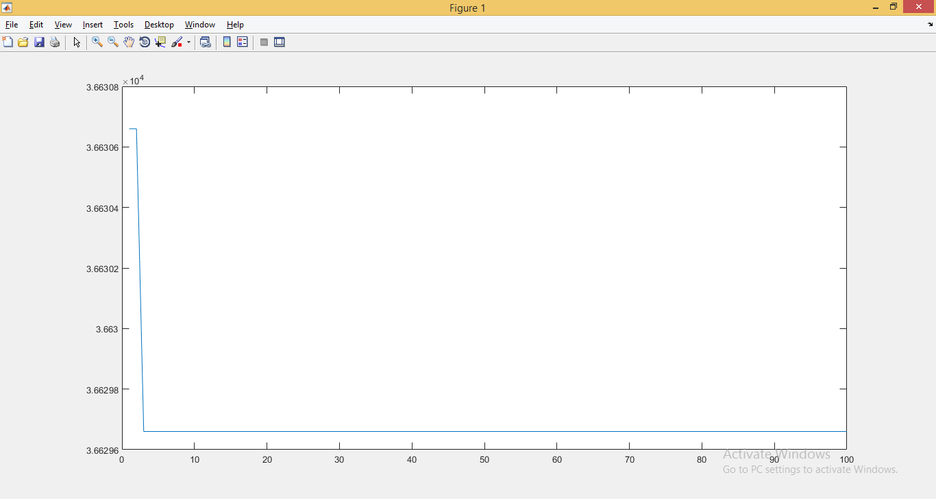
Gradient descent lowered q from 3663.06 to 3662.98 per 100 cycles. Very weak, very unstable.

Test 2. Abatur with default settings.

Now we will run Abatur with standard settings on the same tasks.

1) Regression



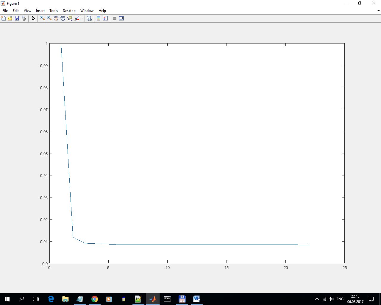
Reduced q from 1 to 0.91 in 20 cycles (in the remaining 80 cycles, he did nothing). Weak, but much stronger than the gradient descent (which lowered from 1.002 to 0.988). And extremely unstable.

2) Quadratic function.



Reduced q from 189 to 179 in 50 cycles (gradient descent lowered q from 140 to about 5). In this situation, Abatur proved to be unstable and ineffective.

3) Discrete function.



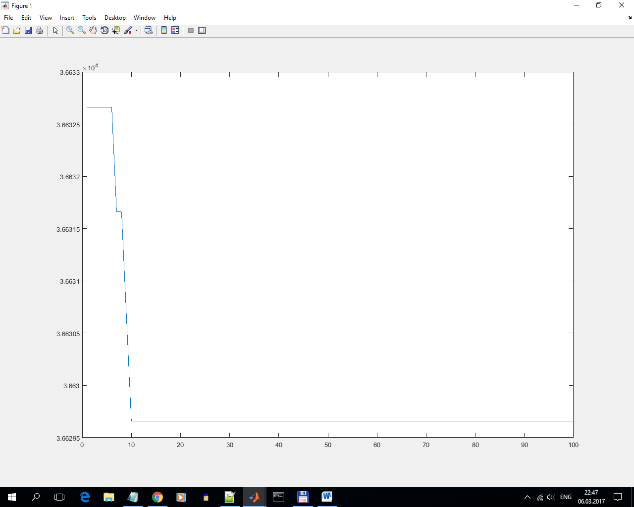
Reduced q from 3663.27 to 3662.98. Very weak, very unstable.

Test 3. Abathur trained.

We teach Abatur on a quadratic function. As a learning algorithm we use Abatur with standard settings.

1) Regression.

The blue lines show the optimization process before learning. Red - after.



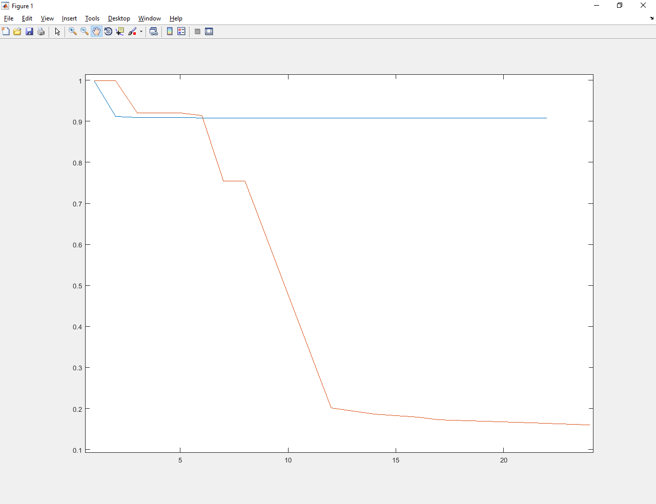
Abathur trained improved the value from about 1 to about 0.17. Much better and the old Abatura, and gradient descent.

2) Quadratic function.



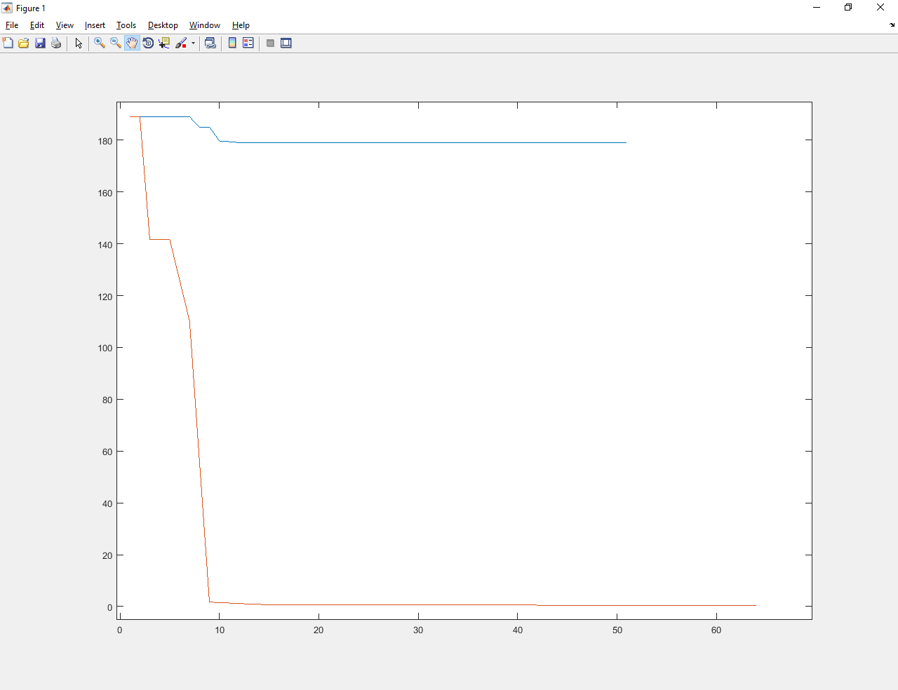
Abathur trained improved the value from about 190 to a number less than 1. Much better than the old Abatura and gradient descent.

3) Discrete function



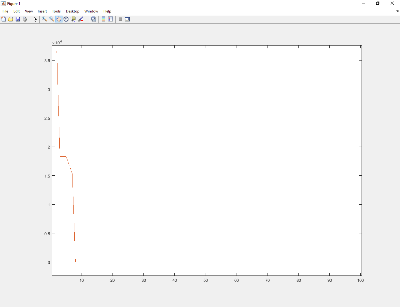
Abathur trained improved the value from about 3,600 to 0.01. Much better and the old Abatura, and gradient descent (which did not cope at all).

Summary

1) Learning optimization algorithm created. The shell for his training is created.
2) I trained Abatur on one task. He became better to solve all the above tasks. Consequently, the algorithm selected heuristics, which in total are suitable for solving any problem from the list.

Sources of literature:

1) “Learning to learn by gradient descent”
2) “Metalearning”