Deep Learning Libraries Theano / Lasagne

Hi, Habr!

In parallel with the publication of open-source machine learning articles, we decided to launch another series - on working with popular frameworks for neural networks and deep learning.

I will open this cycle with an article about Theano, a library that is used to develop machine learning systems both by itself and as a computational backend for higher-level libraries, such as Lasagne , Keras, or Blocks .

Theano has been developed since 2007 mainly by the MILA group from the University of Montreal and is named after the ancient Greek philosopher and mathematician Feano (allegedly depicted in the picture). The main principles are: integration with numpy, transparent use of various computing devices (mainly GPU), dynamic generation of optimized C-code.

We will adhere to the following plan:

• Preface or lyrical digression about libraries for deep learning
• Introduction
  
  • Installation
  • Customization
• The basics
  
  • The first steps
  • Variables and Functions
  • Shared variables and more about functions
  • Debugging
• Machine learning at Theano
  
  • Logistic regression
  • SVM
  • Nonlinear signs
• Lasagne
  
  • Multilayer perceptron
• Conclusion

Code with examples from this post can be found here .

Preface or lyrical digression about libraries for deep learning

Currently, dozens of libraries have been developed for working with neural networks, all of them, sometimes significantly, differ in implementation, but two main approaches can be identified: imperative and symbolic. ^one

Let's look at an example of how they differ. Suppose we want to evaluate a simple expression

$$

$$\ begin {array} {rcl} \ vec a &: = & \ left [10, 10, \ ldots, 10 \ right] ^ T \\ \ vec b &: = & 2 \ cdot \ vec a \\ \ vec c & = & \ vec a \ otimes \ vec b \\ \ vec d & = & \ vec c + 1 \ end {array}$$

This is how it would look in an imperative presentation in python:

a = np.ones(10) b = np.ones(10) * 2 c = b * a d = c + 1 

The interpreter executes the code line by line, storing the results in the variables a , b , c and d .
The same program in the symbolic paradigm would look like this:

  A = Variable('A') B = Variable('B') C = B * A D = C + Constant(1) #   f = compile(D) #  d = f(A=np.ones(10), B=np.ones(10)*2) 

The essential difference is that when we declare D , execution does not occur, we just set the calculation graph, which we then compile and finally execute.

Both approaches have advantages and disadvantages. First of all, imperative programs are more flexible, clearer and easier to debug. We can use all the richness of the programming language used, for example, cycles and branching, display intermediate results for debugging purposes. This flexibility is achieved, first of all, by small restrictions imposed on the interpreter, which should be ready for any subsequent use of variables.

On the other hand, the symbolic paradigm imposes more restrictions, but the calculations are more efficient both in memory and execution speed: at the compilation stage, you can apply a number of optimizations, identify unused variables, perform part of the calculations, reuse memory, and so on. A distinctive feature of symbolic programs is the separate stages of graph declaration, compilation, and execution.

We dwell on it in such detail, because the imperative paradigm is familiar to most programmers, while the symbolic may seem unusual, and Theano is just a clear example of a symbolic framework.

For those who want to understand this issue in more detail, I recommend reading the relevant section of the MXNet documentation (we will write a separate post about this library), but the key point for understanding the rest of the text is that programming with Theano we write to the python program, which then compile and execute.
But enough theory, let's deal with Theano examples.

Installation

For installation, we need: python versions older than 2.6 or 3.3 (better dev version), C ++ compiler (g ++ for Linux or Windows, clang for MacOS), linear algebra library primitives (for example ATLAS, OpenBLAS, Intel MKL), NumPy and SciPy.

To perform computations on a GPU, CUDA will be needed, and a number of operations occurring in neural networks can be accelerated using CuDNN. Starting with version 0.8.0, Theano developers recommend using libgpuarray , which also makes it possible to use multiple GPUs.

When all dependencies are installed, you can install Theano via pip :

 #   pip install Theano #     pip install --upgrade https://github.com/Theano/Theano/archive/master.zip 

Customization

Theano can be configured in three ways:

• Setting the attributes of the theano.config object to the desired value.
• Through the environment variable THEANO_FLAGS
• Through the $HOME/.theanorc configuration file (or $HOME/.theanorc.txt under Windows)

I usually use something like this configuration file:

 [global] device = gpu #  ,       - GPU  CPU floatX = float32 optimizer_including=cudnn allow_gc = False # ,     #exception_verbosity=high #optimizer = None #    #profile = True #profile_memory = True config.dnn.conv.algo_fwd = time_once #         config.dnn.conv.algo_bwd = time_once [lib] Cnmem = 0.95 #   CNMeM (https://github.com/NVIDIA/cnmem) -  CUDA- 

More information about the configuration can be found in the documentation .

The basics

The first steps

Now that everything is installed and configured, let's try to write some code, for example, calculate the value of a polynomial $$$x ^ 2 + 2x + 1$ at point 10:

 import theano import theano.tensor as T #  theano- a = T.lscalar() #   expression = 1 + 2 * a + a ** 2 #  theano- f = theano.function( inputs=[a], #  outputs=expression #  ) #   f(10) >>> array(121) 

Here we performed 4 things: defined a scalar variable type long , created an expression containing our polynomial, defined and compiled the function f , and also executed it, passing the number 10 to the input.

Pay attention to the fact that the variables in Theano are typed, and the type of the variable contains information about both the data type and its dimension, i.e. to calculate our polynomial at several points at once, we need to define as a vector:

 a = T.lvector() expression = 1 + 2 * a + a ** 2 f = theano.function( inputs=[a], outputs=expression ) arg = arange(-10, 10) res = f(arg) plot(arg, res, c='m', linewidth=3.)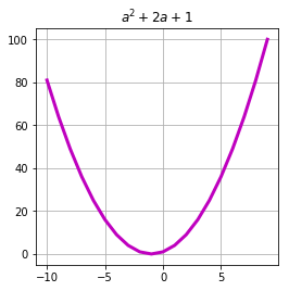 

In this case, we only need to specify the number of dimensions of the variable upon initialization: the size of each dimension is automatically calculated at the stage of the function call.

UPD: It is no secret that the apparatus of linear algebra is universally used in machine learning: examples are described by feature vectors, model parameters are written in the form of matrices, images are presented in the form of 3-dimensional tensors. Scalar quantities, vectors and matrices can be considered as a special case of tensors, therefore, we will call these objects of linear algebra in the future. By a tensor we mean N dimensional arrays of numbers.
theano.tensor package contains the most commonly used types of tensors , however, it is not difficult to determine your type .

If the types do not match, Theano will throw an exception. To fix this, by the way, as well as change much more in the work of functions, you can, by passing the argument allow_input_downcast=True constructor:

 x = T.dmatrix('x') v = T.fvector('v') z = v + x f = theano.function( inputs=[x, v], outputs=z, allow_input_downcast=True ) f_fail = theano.function( inputs=[x, v], outputs=z ) print(f(ones((3, 4), dtype=float64), ones((4,), dtype=float64)) >>> [[ 2. 2. 2. 2.] >>> [ 2. 2. 2. 2.] >>> [ 2. 2. 2. 2.]] print(f_fail(ones((3, 4), dtype=float64), ones((4,), dtype=float64)) >>> --------------------------------------------------------------------------- >>> TypeError Traceback (most recent call last) 

We can also evaluate several expressions at once, the optimizer in this case can reuse intersecting parts, in this case the sum $$$x + y$ :

 x = T.lscalar('x') y = T.lscalar('y') square = T.square(x + y) sqrt = T.sqrt(x + y) f = theano.function( inputs=[x, y], outputs=[square, sqrt] ) print(f(5, 4)) >>> [array(81), array(3.0)] print(f(2, 2)) >>> [array(16), array(2.0)] 

For the exchange of states between functions, special shared variables are used:

 state = theano.shared(0) i = T.iscalar('i') inc = theano.function([i], state, #    updates=[(state, state+i)]) dec = theano.function([i], state, updates=[(state, state-i)]) #         print(state.get_value()) inc(1) inc(1) inc(1) print(state.get_value()) dec(2) print(state.get_value()) >>> 0 >>> 3 >>> 1 

The values ​​of such variables, as opposed to tensor variables, can be obtained and modified outside of the Theano-functions from the usual python-code:

 state.set_value(-15) print(state.get_value()) >>> -15 

Values ​​in shared variables can be “substituted” in tensor variables:

 x = T.lscalar('x') y = T.lscalar('y') i = T.lscalar('i') expression = (x - y) ** 2 state = theano.shared(0) f = theano.function( inputs=[x, i], outputs=expression, updates=[(state, state+i)], #    state    y givens={ y : state } ) print(f(5, 1)) >>> 25 print(f(2, 1)) >>> 1 

Debugging

Theano provides a variety of tools to display a graph of computation and debugging. However, debugging symbolic expressions is still not an easy task. We briefly list the most commonly used approaches here, for more information on debugging, see the documentation: http://deeplearning.net/software/theano/tutorial/printing_drawing.html

We can print a calculation graph for each function:

 x = T.lscalar('x') y = T.lscalar('y') square = T.square(x + y) sqrt = T.sqrt(x + y) f = theano.function( inputs=[x, y], outputs=[square, sqrt] ) #       theano.printing.debugprint(f) 

Note that the amount is calculated only once:

 Elemwise{Sqr}[(0, 0)] [id A] '' 2 |Elemwise{add,no_inplace} [id B] '' 0 |x [id C] |y [id D] Elemwise{sqrt,no_inplace} [id E] '' 1 |Elemwise{add,no_inplace} [id B] '' 0 

Expressions can also be displayed in a more concise form:

 #   W = T.fmatrix('W') b = T.fvector('b') X = T.fmatrix('X') expr = T.dot(X, W) + b prob = 1 / (1 + T.exp(-expr)) pred = prob > 0.5 #    theano.pprint(pred) >>> 'gt((TensorConstant{1} / (TensorConstant{1} + exp((-((X \\dot W) + b))))), TensorConstant{0.5})' 

Or in the form of a graph:

 theano.printing.pydotprint(pred, outfile='pics/pred_graph.png', var_with_name_simple=True)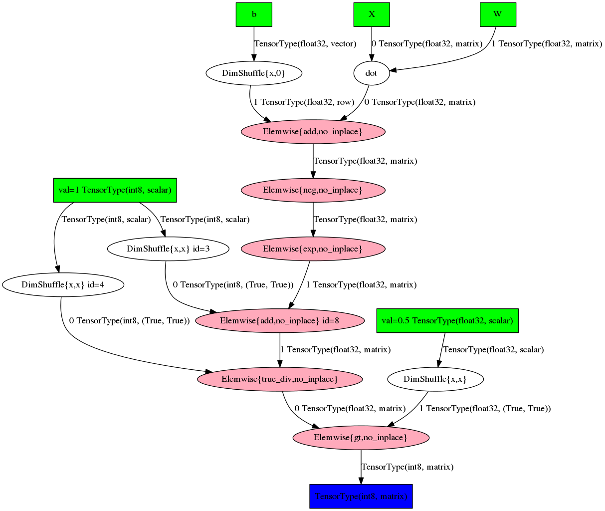 

Unfortunately, the readability of such graphs drops sharply with increasing complexity of expression. In fact, something can only be understood through toy examples.

Machine learning at Theano

Logistic regression

Let's look at the example of logistic regression, how you can develop machine learning algorithms using Theano. Intentionally, we will not go into details of how this model is structured (let's leave it until the corresponding article in the open course), but recall that the posterior probability of the class $$$C_1$ has the appearance $$$p (C_1 | X) = \ hat {y} = \ sigma (w ^ TX + b)$

Let's define the parameters of the model, for convenience, we introduce a separate parameter for the offset:

 W = theano.shared( value=numpy.zeros((2, 1),dtype=theano.config.floatX), name='W') b = theano.shared( value=numpy.zeros((1,), dtype=theano.config.floatX), name='b') 

And we will get character variables for attributes and class labels:

 X = T.matrix('X') Y = T.imatrix('Y') 

Let's now define the expressions for the posterior probability and the model predictions:

 linear = T.dot(X, W) + b p_y_given_x = T.nnet.sigmoid(linear) y_pred = p_y_given_x > 0.5 

And we define the loss function of the form: $$$L = - \ frac {1} {N} \ sum_ {n = 1} ^ {N} [y \ log {\ hat {y}} + (1-y) \ log {(1 - \ hat {y })}]$

 loss = T.nnet.binary_crossentropy(p_y_given_x, Y).mean() 

We did not explicitly write out the expressions for sigmoids and cross-entropies explicitly, but used the functions from the theano.tensor.nnet package, which provides optimized implementations of a number of functions popular in machine learning. In addition, features from this package usually include additional tricks for numerical stability.

To optimize the loss function, let's use the gradient descent method, each step of which is given by the expression:

$$

$$\ large w_ {n + 1} = w_n - \ eta \ frac {1} {n} \ nabla E (w_n)$$

Let's put it in code:

 g_W = T.grad(loss, W) g_b = T.grad(loss, b) updates = [(W, W - 0.04 * g_W), (b, b - 0.08 * g_b)] 

Here we used the wonderful opportunity of Theano - automatic ² differentiation. The call to T.grad returned to us an expression that would contain the gradient of the first argument in the second. This may seem redundant for such a simple case, but it helps a lot when building large, multi-layered models.

When the gradients are obtained, we just need to compile the Theano functions:

 train = theano.function( inputs=[X, Y], outputs=loss, updates=updates, allow_input_downcast=True ) predict_proba = theano.function( [X], p_y_given_x, allow_input_downcast=True ) 

And run an iterative process:

 sgd_weights = [W.get_value().flatten()] for iter_ in range(4001): loss = train(x, y[:, np.newaxis]) sgd_weights.append(W.get_value().flatten()) if iter_ % 100 == 0: print("[Iteration {:04d}] Train loss: {:.4f}".format(iter_, float(loss))) 

For the data I generated, the process converges to this dividing line: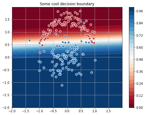

It looks good, but it seems that for such a simple task, 4000 iterations are a bit too much ... Let's try to speed up the optimization and use the Newton method . This method uses the second derivatives of the loss function and is a sequence of such steps:

$$

$$\ large w_ {n + 1} = w_n - H ^ {- 1} \ nabla E (w_n)$$

Where $$$H$ - Hesse matrix.

To calculate the Hessian matrix, create one-dimensional versions of the parameters of our model:

 W_init = numpy.zeros((2,),dtype=theano.config.floatX) W_flat = theano.shared(W_init, name='W') W = W_flat.reshape((2, 1)) b_init = numpy.zeros((1,), dtype=theano.config.floatX) b_flat = theano.shared(b_init, name='b') b = b_flat.reshape((1,)) 

And we define the optimizer step:

 h_W = T.nlinalg.matrix_inverse(theano.gradient.hessian(loss, wrt=W_flat)) h_b = T.nlinalg.matrix_inverse(theano.gradient.hessian(loss, wrt=b_flat)) updates_newton = [(W_flat, W_flat - T.dot(h_W , g_W)), (b_flat, b_flat - T.dot(h_b, g_b))] 

Although we have come to the same results,
,
Newton's method required only 30 steps (against 4000 at the gradient descent).

The ways of both methods can be viewed on this chart: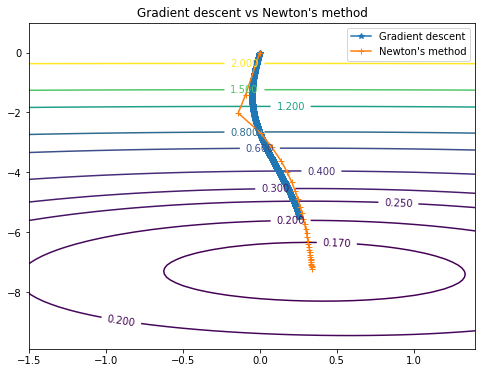

Svc

We can also easily implement the support vector method, for this it is enough to present the loss function in the following form:

$$

$$\ large C \ sum_ {n = 1} ^ {N} [1 - w ^ T \ phi (x) + b] _ + + || w || ^ 2$$

In terms of Theano, this can be written by replacing several lines in the previous example:

 C = 10. loss = C * T.maximum(0, 1 - linear * (Y * 2 - 1)).mean() + T.square(W).sum() predict = theano.function( [X], linear > 0, allow_input_downcast=True ) 

$$$C$ this is a hyperparameter that regularizes the model, and the expression $$$(Y * 2 - 1)$ just translates tags into a range $$$\ {- 1, 1 \}$

For selected C, the classifier will divide the space as follows:

Nonlinear signs

Cycles are one of the most commonly used constructs in programming. Cycle support in Theano is provided by the scan function Let's get acquainted with how it works. I think it is already obvious to readers that the linear function of the signs is not the best candidate for the separation of the generated data. This disadvantage can be corrected by adding polynomial signs to the original ones (this technique is described in detail in another article of our blog). So, I want to get a view conversion $$$\ {x_1, x_2 \} \ rightarrow \ bigcup \ limits_ {i = 0} ^ {i = K} \ {x_1 ^ i, x_2 ^ i \}$ . In python, we could implement it, for example, like this:

 poly = [] for i in range(K): poly.extend([x**i for x in features]) 

In Theano, it looks like this:

 def poly(x, degree=2): result, updates = theano.scan( #  ,      fn=lambda prior_result, x: prior_result * x, #    outputs_info=T.ones_like(x), # ,  x       fn non_sequences=x, #   n_steps=degree) #      N x M*degree return result.dimshuffle(1, 0, 2).reshape((result.shape[1], result.shape[0] * result.shape[2])) 

The first in scan is the function that will be called at each iteration, its first argument is the result at the previous iteration, the next are all non_sequences ; outputs_info initializes the output tensor of the same dimension and type as x , and fills it with units; n_steps indicates the required number of iterations.

scan will return the result in the form of a size tensor (n_steps, ) + outputs_info.shape , so we will convert it into a matrix in order to get the necessary attributes.

We illustrate the operation of the resulting expression with a simple example:

 [[1, 2], -> [[ 1, 2, 1, 4], [3, 4], -> [ 3, 4, 9, 16], [5, 6]] -> [ 5, 6, 25, 36]] 

To reap the benefits of your efforts, it is enough to change the definition of the model and add parameters (there are more signs):

 W = theano.shared( value=numpy.zeros((8, 1),dtype=theano.config.floatX), name='W') linear = T.dot(poly(X, degree=4), W) + b 

New features make it much better to divide classes: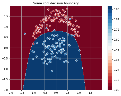

Neural Networks and Lasagne ³

At this point, we have already discussed the main stages of creating Theano machine learning systems: initializing input variables, defining a model, compiling Theano functions, a cycle with optimizer steps. This could be the end of it, but I really want to acquaint readers with Lasagne - a wonderful library for neural networks running on top of Theano. Lasagne provides a set of ready-made components: layers, optimization algorithms, loss functions, initialization of parameters, etc., while not hiding Theano behind numerous layers of abstractions.

Consider what a typical code on Theano / Lasagne might look like using the MNIST classification as an example .

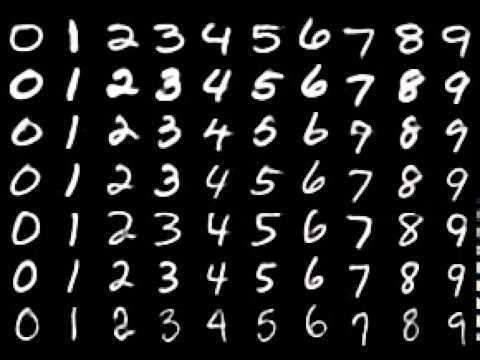
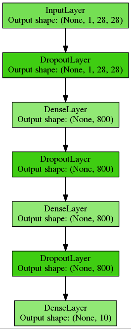
We construct a multilayer perceptron with two hidden layers of 800 neurons each, for regularization we will use a dropout and place this code in a separate function:

 def build_mlp(input_var=None): #  ,    # (  minibatch'a, 1 , 28   28 ) #        , #        network = lasagne.layers.InputLayer( shape=(None, 1, 28, 28), input_var=input_var) # dropout  20%    network = lasagne.layers.DropoutLayer(network, p=0.2) #    800   ReLU    #    ,  Xavier Glorot  Yoshua Bengio network = lasagne.layers.DenseLayer( network, num_units=800, nonlinearity=lasagne.nonlinearities.rectify, W=lasagne.init.GlorotUniform()) #  dropout   50%: network = lasagne.layers.DropoutLayer(network, p=0.5) #      network = lasagne.layers.DenseLayer( network, num_units=800, nonlinearity=lasagne.nonlinearities.rectify) network = lasagne.layers.DropoutLayer(network, p=0.5) # ,    10 : network = lasagne.layers.DenseLayer( network, num_units=10, nonlinearity=lasagne.nonlinearities.softmax) return network 

We get just such a simple mesh network:

Initialize the tensor variables and compile the Theano functions for learning and validation:

 input_var = T.tensor4('inputs') target_var = T.ivector('targets') #      network = build_mlp(input_var) #      ,   prediction = lasagne.layers.get_output(network) #    loss = lasagne.objectives.categorical_crossentropy(prediction, target_var).mean() #     L1  L2 , . lasagne.regularization. #        #    keyword ,      #     trainable  regularizable params = lasagne.layers.get_all_params(network, trainable=True) #         updates = lasagne.updates.nesterov_momentum( loss, params, learning_rate=0.01, momentum=0.9) #        . #       deterministic=True, #   dropout test_prediction = lasagne.layers.get_output(network, deterministic=True) test_loss = T.nnet.categorical_crossentropy(test_prediction, target_var).mean() #     test_acc = T.mean( T.eq(T.argmax(test_prediction, axis=1), target_var), dtype=theano.config.floatX) #     train = theano.function( inputs=[input_var, target_var], outputs=loss, updates=updates) #   —   #  Theano  ,        #      validate = theano.function( inputs=[input_var, target_var], outputs=[test_loss, test_acc]) 

Now create a learning cycle:

 print("| Epoch | Train err | Validation err | Accuracy | Time |") print("|------------------------------------------------------------------------|") try: for epoch in range(100): #         train_err = 0 train_batches = 0 start_time = time.time() for batch in iterate_minibatches(X_train, y_train, 500, shuffle=True): inputs, targets = batch train_err += train(inputs, targets) train_batches += 1 #     val_err = 0 val_acc = 0 val_batches = 0 for batch in iterate_minibatches(X_val, y_val, 500, shuffle=False): inputs, targets = batch err, acc = validate(inputs, targets) val_err += err val_acc += acc val_batches += 1 print("|{:05d} | {:4.5f} | {:16.5f} | {:10.2f} | {:7.2f} |".format (epoch, train_err / train_batches, val_err / val_batches, val_acc / val_batches * 100, time.time() - start_time)) except KeyboardInterrupt: print("The training was interrupted on epoch: {}".format(epoch)) 

The resulting learning curves:

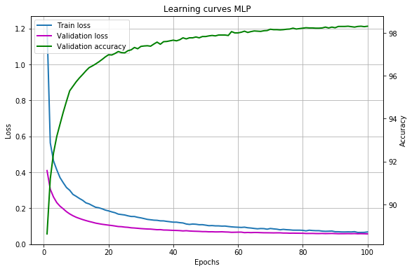
Our model achieves an accuracy of more than 98%, which can undoubtedly be improved using, for example, convolutional neural networks, but this topic is already beyond the scope of this article.

It is convenient to save and load weights with the help of helpers:

 #   savez('model.npz', *lasagne.layers.get_all_param_values(network)) network = build_mlp() #  ,  : with np.load('model.npz') as f: param_values = [f['arr_%d' % i] for i in range(len(f.files))] lasagne.layers.set_all_param_values(network, param_values) 

Documentation for Lasagne is available here , a lot of examples and pre-trained models are in a separate repository .

Conclusion

In this post, we are quite superficially acquainted with the possibilities of Theano, you can learn more:

• referring to the documentation: 1 , 2
• looking at code samples
• communicating with the community
• looking at the source code .

Big thanks to bauchgefuehl for help in preparing the post.

---

1. The border between the two approaches is rather blurred, and not everything said below is strictly true, there are always exceptions and borderline cases. Our task here is to convey the main idea.
2. The Theano developers in the technical report and documentation call character differentiation.However, the use of this term in one of the previous articles on Habr caused a discussion. Based on the Theano source code and the definition on Wikipedia, the author believes that the correct term is still “automatic differentiation”.
3. The material in this section is mostly based on Lasagne documentation .