I wrote the fastest hash table

In the end I had to come to this. Once I published an article " I wrote a fast hash table, " and then another one, " I wrote an even faster hash table ." Now I have completed the fastest hash table. And by this I mean that I implemented the fastest search compared to all the hash tables I could find. At the same time, insert and delete operations also work very quickly (although not faster than competitors).

I used Robin Hood hashing with a limit on the maximum number of sets. If an element should be at a distance more than X positions from its ideal position, then we increase the table and hope that in this case each element can be closer to its desired position. This approach seems to work really well. The value of X may be relatively small, which allows for some optimization of the internal search cycle on the hash table.

If you only want to try it at work, you can download it from here . Or scroll down to the “Source Code and Usage” section. Want details - read on.

Hash Table Type

There are many types of hash tables. For my, I chose:

• Open Addressing.
• Linear placement.
• Hashing Robin Hood.
• The number of slots is a prime number (but I realized the possibility of using numbers for this purpose, which are powers of two).
• Limit the maximum number of sets.

I think the last point is a novelty in the field of hash tables. This is the main reason for the high performance of my solution. But first I would like to talk about the previous points.

Open addressing means that the hash table uses a continuous array as data storage. This is not an analogue of std::unordered_map , when each element is in a separate heap.

Linear placement means that if you try to insert an element into an array, and the current slot is already full, then you simply go to the next slot. If it is also filled, then the next slot is taken, and so on. This simple approach has known flaws, but I believe that they are corrected by limiting the maximum number of sets.

Hashing Robin Hood means that with linear placement you try to position each element as close as possible to its ideal position. This is done by moving the surrounding elements when inserting or deleting an element. The principle is this: we take from rich elements (rich elements) and transfer to poor elements (poor elements). Hence the name Robin Hood. An element that has received a slot in the vicinity of its ideal insertion point is called rich. The poor element is far away from the ideal insertion point. By inserting a new element, you count how far it is from the ideal position. If it is further than the current element, then you put a new one in place of the current one, and then try to find a new place for it.

The number of slots is a prime number : the size of the array underlying the hash table is a prime number. This means that it can grow, for example, from 5 slots to 11, then to 23, to 47, and so on. When you need to find the insertion point, then the modulo operator is used to assign the element's hash value to the slot. Another option is to make the size of the array equal to the power of two. Below we will talk about why by default I use simple numbers and when it is advisable to use both options.

Limit the maximum number of sets

We've figured out the basics, let's now discuss my solution: limiting the maximum number of slots in which the table will perform a search, after which it spits and increases the size of the array.

First, the idea was to make this number very small, for example, equal to 4. That is, when inserting, I first try the perfect slot, if it does not work, then I turn to the next, then to the next, then to the next, and if all of them are filled then I enlarge the table and try again to insert the element. This works great on small tables. But when I insert a random value into a large table, I will always fail with these four sets; I will have to increase the size of the table, even if it is mostly empty.

In the end, I found that with the upper limit equal to log2 (n), where n is the number of slots in the table, reallocation is performed only when it is approximately 2/3 full. This is when inserting a random value. And if you insert consecutive values, then you can fill the table as a whole, and only then it will be redistributed.

But despite the empirically found threshold of 2/3, from time to time the redistribution was launched at 60% of the table filling. Occasionally - even at 55% m. Therefore, I assigned a max_load_factor table value of 0.5. This means that the table will increase when filled to 50%, even if the limit on the number of sets has not been reached. I did this so that you can trust the table redistribution, when you really increase its size: if you insert a thousand items, then delete a couple of them, and then insert the same number again, you can be almost completely sure that the table will not be redistributed. I do not have exact statistics, but I drove a simple test in which I built thousands of tables of various sizes and filled them with random numbers. In sum, I performed the insertion of hundreds of billions of numbers, and only once was the redistribution with a load factor (less than 0.5) (the table increased when filling 48%). So you can trust such a mechanism: it very rarely redistributes when you don’t wait.

In general, if you do not need to control the increase in the table, freely max_load_factor value higher. Safely set up to 0.9: high speed of all operations is provided by a combination of Robin Hood and restrictions on the number of sets. But do not assign a value of 1.0: a situation may arise when, when inserting, the movement of each element of the table begins to fill the last remaining slot. For example, all slots in which the last element wants to be are already occupied, except for the last empty one. Then you insert the element in the first slot in which he wants to be, but he is already busy. You will have to move the existing element to the second slot, from there evict the element to the third, and so on by the chain to the end of the table. As a result, you get a table in which all the elements, with the exception of the very first one, are in one slot from their ideal positions. The search will still be fast, but the last insertion will take a long time. If you have several free slots nearby, then the inserted element will move not so many neighbors.

If you set max_load_factor such a low value that the limit on the number of sets will never be reached, then why limit anything at all? Thanks to this limitation, you can implement a fine optimization: let's say you re-cache the table to get 1000 slots. In my case, the table will grow to 1009, this is the nearest prime number. The binary logarithm of 1009 is rounded to 10, so I limit the number of sets to ten. Now apply the trick: instead of an array on 1009 slots, we will create an array on 1019. But all other hashing operations will assume that we have only 1009 slots. Now, if two elements are hashed into the index 1008, then I can go to the end and insert into the index 1009. I do not need to check the range of indexes (bounds checking), because limiting the number of sets will not let me go beyond the index 1018. If If there are 11 elements that I want to get into the last slot, then the table will increase and all these elements will be combined into different slots. Due to the absence of boundary checking, I have compact inner loops. Here’s what the search function looks like:

 iterator find(const FindKey & key) { size_t index = hash_policy.index_for_hash(hash_object(key)); EntryPointer it = entries + index; for (int8_t distance = 0;; ++distance, ++it) { if (it->distance_from_desired < distance) return end(); else if (compares_equal(key, it->value)) return { it }; } } 

In essence, this is a linear search. The code is beautifully converted to assembler. This approach is better than simple linear placement for two reasons:

1. There is no check of the range of variation of indices. Empty slots have a distance_from_desired value of –1, so this is similar to finding another item.
2. In the loop, no more log2 (n) iterations are performed. Usually when searching in hash tables, the worst time complexity is O (n). In my table - O (log n). This is a big difference. Especially given the fact that with linear placement, the worst option is preferable, since the elements tend to be grouped.

My memory overhead is 1 byte per item. I store distance_from_desired in int8_t . That is, when aligning the type (alignment of the type) of the inserted element will be padded (padded out) 1 byte. So if you insert integer values, then 1 byte will receive another 3 bytes of padding, resulting in 4 bytes of overhead for each element. If you insert pointers, then padding will be already 7 bytes, we get 8 bytes of overhead. To solve this problem, I am considering the option of changing the memory usage scheme, but I fear that then I will have two cache misses for each search instead of one. So the memory overhead is 1 byte per element + padding. And with the max_load_factor value max_load_factor to 0.5, your table will be filled only by 25–50%, so the total overhead is even higher. Let me remind you that, in order to save memory, you can safely increase max_load_factor to 0.9, this will only lead to a slight decrease in speed.

Search performance

It’s not so easy to figure out the performance of hash tables. At a minimum, you need to measure speed in such situations:

1. Search for an item in a table.
2. Search for an element that is not in the table.
3. Insert a group of random numbers.
4. Inserts a group of random numbers after calling reserve() .
5. Removing items.

And each of these situations needs to be run with different keys and values ​​of different sizes. I use an integer or string value as a key, and 4, 32, and 1024 value types. I prefer integer values, because with string values ​​you mostly measure the overhead of the hash function and the comparison operator, the same for all hash tables.

It is necessary to test the search both in the presence of an element in the table, and in its absence, because in these cases the performance can be completely different. For example, I faced a difficult situation when I inserted all the numbers from 0 to 500,000 into google::dense_hash_map (not random numbers), and then I searched for the missing element. Unexpectedly, the hash table is 500 times slower than usual. This is an extreme case - using the power of two to set the size of the table. Probably, it was necessary to take measurements with random numbers and with consecutive ones, but then there would be too many graphs. So I will confine myself to random numbers, they eliminate the occurrence of unsuccessful performance situations due to specific patterns.

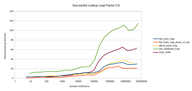
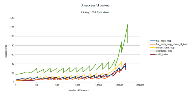
The first chart is the search for an element present in the table:

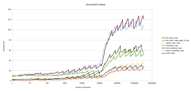
The graphics are pretty tight. flat_hash_map is my new hash table. flat_hash_map_power_of_two is the same table, but the size of the array is determined by a power of two, not a prime number. As you can see, the second option is much faster, I will explain the reason later. dense_hash_map is google::dense_hash_map , the fastest hash table I found. sherwood_map is the old table from “I wrote a faster hash table”. To my confusion, she showed mediocre results ... std::unordered_map and boost::unordered_map - everything is clear from the names. multi_index is boost::multi_index .

We will discuss this schedule a bit. Y axis - the number of nanoseconds spent on the search for a single element. I used Google Benchmark, which call the table.find() function time after time, and then it calculates how many times it has been able to do it. The total duration of the iterations is divided by their number, resulting in nanoseconds. All required keys are present in the table. For the X axis, I took the logarithmic scale, because it describes well the change in performance. In addition, this scale allows us to estimate the performance for tables of different sizes: if you are interested in small tables, then look at the left side of the graph.

Immediately striking jagged graphs. The point is that all the tables have different performance depending on the current fill factor (load factor), that is, the degree of filling. At 25%, the search will be performed faster than at 50%: the larger the table, the more hash collisions occur. The cost of the search grows, and at some point the table decides that it has filled too much and it is time to reallocate, which again results in faster search.

This would be obvious if I displayed the fill factor graphs for each table. Also, you would immediately see that the lower graphs are obtained at max_load_factor , equal to 0.5, and the upper ones - at 1.0. The question immediately arises: would the tables in the upper graphs be faster than the lower ones for the same value - 0.5? There would be, but very slightly. Next we look at this situation more fully. The graph shows that the lower point of the upper graphs, when the tables have just been redistributed and have a fill factor of just over 0.5, is located much higher than the upper point of the lower graphs just before the redistribution, due to the fact that their fill factor approaches 0.5 .

You also see that on the left side all the graphs are relatively flat. The reason is that the tables are completely sent to the cache. Only when the data ceases to fit in the L3 cache does the graphics noticeably diverge. I think this is a big problem. In my opinion, the right side of the graphs reflects the situation much more accurately than the left one: you will get results similar to the left side only when the desired item is already in the cache.

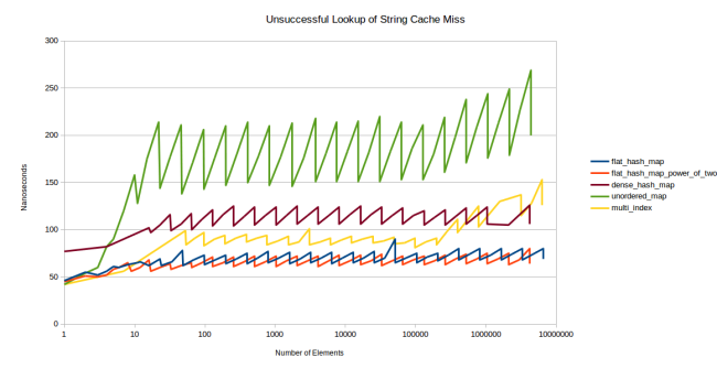
Therefore, I tried to come up with a test that would show the speed of the table, which is not in the cache. I created so many tables so that they did not fit in L3, and used different tables for each element sought. Suppose I want to measure the speed of a table containing 32 elements of 8 bytes each. The size of my L3 cache is 6 MB, so approximately 25 thousand such tables fit into it. To make sure that the tables in the cache are missing, I created them with a margin of 75 thousand pieces. And each search was performed in a separate table.

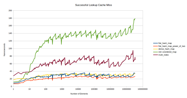
I removed a couple of lines, because they were uninformative. boost::unordered_map and std::unordered_map usually show the same performance, and no one cares about my old slow sherwood_map table. Now we have left: std::unordered_map as a regular container based on nodes (node ​​based container), boost::multi_index as a fast container based on nodes (I think that std::unordered_map can be no less fast), google::dense_hash_map as a fast open addressing container and my new container in two versions - based on prime numbers and powers of two.

In the new benchmark graphics immediately began to vary greatly. The pattern that appeared on the graph of the first benchmark on the graph of the second benchmark became noticeable very early, starting with 10 elements. Impressive: all tables show stable performance in a very large range of the number of elements.

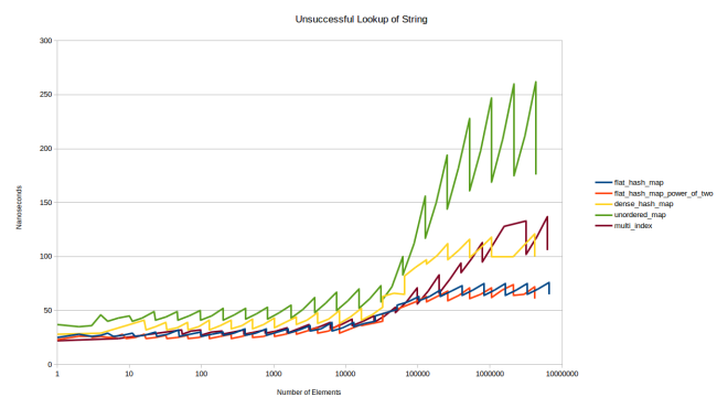
Let's look at the charts of a failed search — that is, a search for an element that is not in the table.

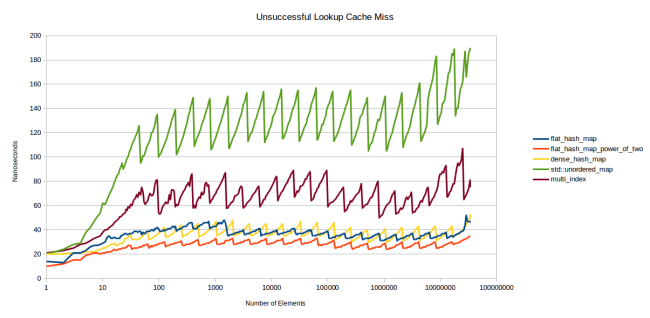
Serration is even more pronounced, the fill factor plays a prominent role. The stronger the table is, the more elements you have to look through before the system decides that the element is missing. But I really like the results of my table: it looks like the limit on the number of sets works. My table shows more stable performance than others.

These graphs convinced me that my new table is a big step forward. The red line shows the operation of my table, configured in the same way as dense_hash_map: max_load_factor 0,5 , and the choice to determine the size of a power of two allows you to place a hash in the slot simply by the dense_hash_map: max_load_factor 0,5 bits. The only big difference: my table uses an extra byte for storage (plus padding) for each slot, that is, it consumes slightly more memory than dense_hash_map .

At the same time, my table is not inferior in speed even when using simple numbers to determine the size of the table. Let's talk about this in more detail.

Prime numbers or power of two

Finding an item in a table goes through three expensive steps:

1. Key Hashing
2. Placement of the key in the slot.
3. Getting memory for this slot.

Stage 1 can be cheap if the key is an integer: just drop it in size_t . But with other types of keys, such as string, the stage will be more expensive.

Stage 2 - integer modulo.

Stage 3 - pointer dereference. In the case of std::unordered_map this is a dereferencing of several pointers.

It may seem that if you have a not too slow hash function, then stage 3 is the most expensive of all. But if you do not have cache misses on every single search, then the second is most likely the most expensive step. The integer modulo is processed slowly, even on powerful hardware. According to Intel , this takes from 80 to 95 cycles.
This is the main reason why really fast hash tables usually use a power of two to determine the size of the array. Because then it will be enough for you to remove the high bits, which can be done in one cycle.

But the power of two has a big drawback: quite a few patterns of input data create numerous collisions of hashes when using a power of two. Here is a graph of the second benchmark, but this time I did not use random numbers:

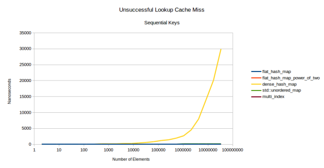
Yes, that's right: google::dense_hash_map went into the stratosphere. For this, it was enough to give her a set of numbers in order: [0, 1, 2, ..., n - 2, n - 1]. If you do this and look for a key that is not in the table, the search will be extremely slow. If there is a key, then everything is fine, it works quickly. In this case, the difference in performance between successful and unsuccessful search can reach thousands of times.

Another example of the problem is due to the power of two: the standard hash table in Rust began to demonstrate quadratic behavior (quadratic) when inserting keys from one table to another. So using a power of two can lead to unpleasant surprises.

It so happened that my table avoided all these problems by limiting the number of sets. There was not even unnecessary redistribution. But this does not mean that my table is invulnerable to side effects of using a power of two. For example, I somehow came across the fact that when inserting pointers into such a table, some slots were constantly empty. , 16- , -, reinterpret_casted size_t . - . -.

, -, . : -. , . , , . ( ).

? , , , . , , 32 , 16- ( 16). : 0 16. 32 16, . , . , 37 , 16 37 .

? boost::multi_index : (compile time constant). . , . . - , :

 switch(prime_index) { case 0: return 0llu; case 1: return hash % 2llu; case 2: return hash % 3llu; case 3: return hash % 5llu; case 4: return hash % 7llu; case 5: return hash % 11llu; case 6: return hash % 13llu; case 7: return hash % 17llu; case 8: return hash % 23llu; case 9: return hash % 29llu; case 10: return hash % 37llu; case 11: return hash % 47llu; case 12: return hash % 59llu; // // ...   // case 185: return hash % 14480561146010017169llu; case 186: return hash % 18446744073709551557llu; } 

— . What is good? , . , , . , .

: , -, . , . , std::map . , , . , .

. - , . ? , - -, , . - . , , dense_hash_map , , , .

, . : , , , . . -, , . , - , , std::hash -, (stateful), . , , , .

, , , - , . . typedef hash_policy -. , .

, typedef -:

 struct CustomHashFunction { size_t operator()(const YourStruct & foo) { //  - } typedef ska::power_of_two_hash_policy hash_policy; }; // : ska::flat_hash_map<YourStruct, int, CustomHashFunction> your_hash_map; 

- hash_policy ska::power_of_two_hash_policy . flat_hash_map . std::hash , power_of_two_std_hash , std::hash , power_of_two_hash_policy :

 ska::flat_hash_map<K, V, ska::power_of_two_std_hash<K>> your_hash_map; 

-, , .

. , . , N , . reserve() :

, . , . , .

, , L3. , , , — .

google::dense_hash_map , . , dense_hash_map . . Robin Hood , « ». . , .

, , reserve() :

, . , . , malloc (Linux gcc). , .

, - , reserve . , , google::dense_hash_map .

, . N . N:

, . 23 , dense_hash_map — 20. .

: dense_hash_map , «» (tombstone). , . «» (quadratic probing), google::dense_hash_map : , . Robin Hood , : , . , . . «», . .

, «», . dense_hash_map . , , : :

. -, , . . , : 1, 2, 3 4. «, , » : 1, 3, 1, 2, 4, 4, 4, 1, 2, 3, 3, 2. , , . . — . — , ( ). — , , , , . . And so on.

dense_hash_map , . , — . 6 . , , . , 500 . . --, . , dense_hash_map «», . dense_hash_map :

, dense_hash_map , «». . Robin Hood : , . , .

max_load_factor()

, std::unordered_map boost::multi_index max_load_factor, 1,0, google::dense_hash_map 0,5. max_load_factor ? , ( ), max_load_factor 0,5. .

, max_load_factor 0,5, , , . , , . , , - , max_load_factor .

flat_hash_map dense_hash_map , . , dense_hash_map , : L3, flat_hash_map .

boost::multi_index std::unordered_map , max_load_factor 1,0, flat_hash_map dense_hash_map , max_load_factor — 0,5. , flat- .

, , . , -, . , max_load_factor . , , - . — . : .

(map from int to int). . — :

, . . , . , - . :

: , google::dense_hash_map , boost::multi_index . : dense_hash_map , , , «». , , std::string(1, 0) std::string(1, 255) . , , , . .

, . , . , . :

, dense_hash_map ( ). .

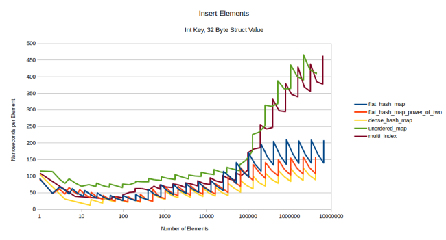
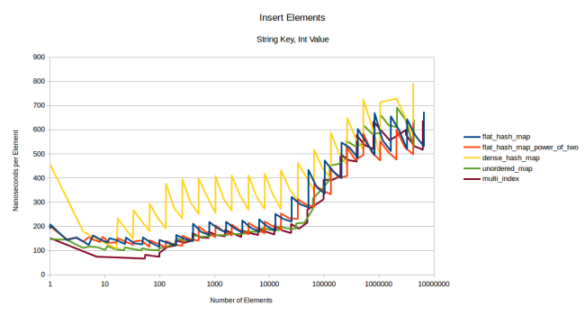
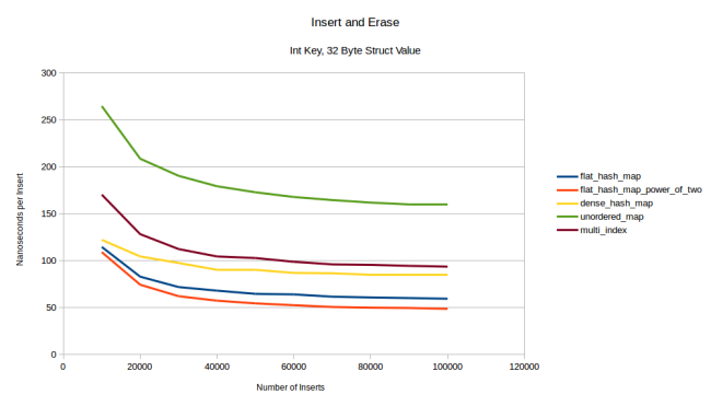
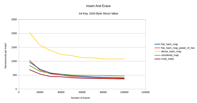
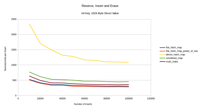
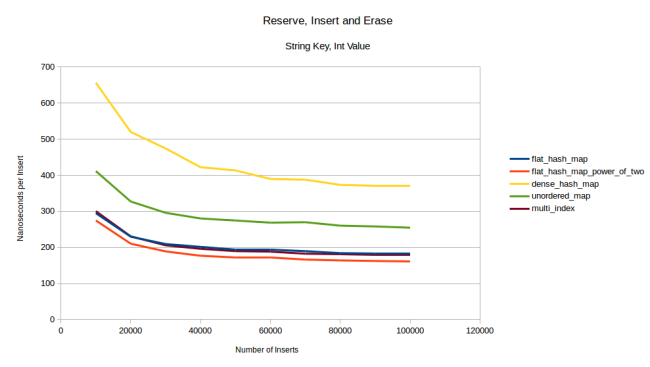
. (map from int to int), 32- ? 1024- ? 12 ([, 32-, 1024-] × [, ] × [ , ]), , : , . : 1024- :

, 1024- multi_index flat-. , , - prefetcher . , 1024 .

, : . flat- . max_load_factor 0,5, . : , , . , — . , (prefetch) .

(size of the type), . 32- :

, flat-, : , . , boost::multi_index . , 1024- :

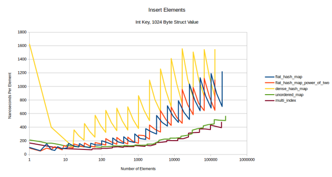
: flat- , , . .

: dense_hash_map ( ). , 32 - (default constructed value type). - — 1024 , 32 . , , .

dense_hash_map . , , -, - , , .

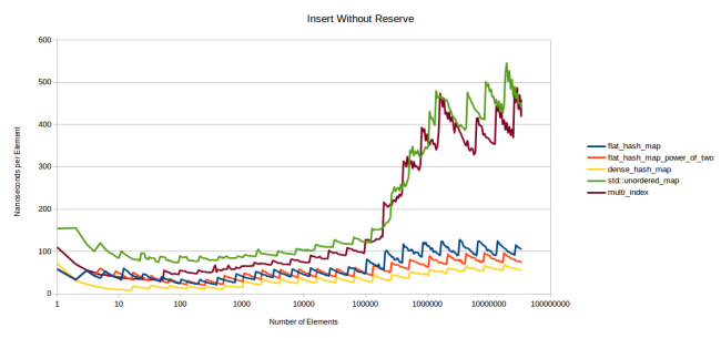
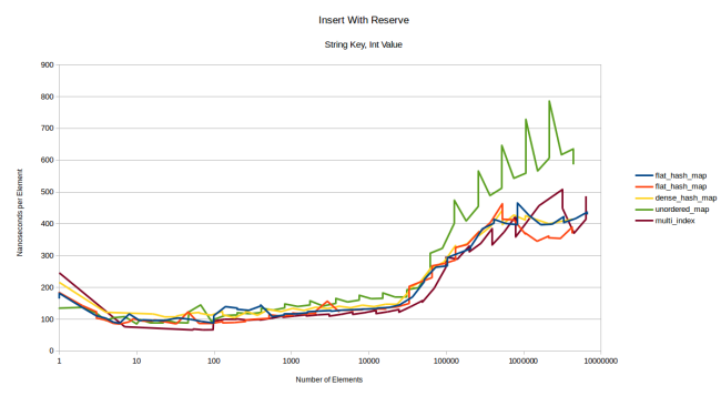
, , , reserve() . , , , reserve() :

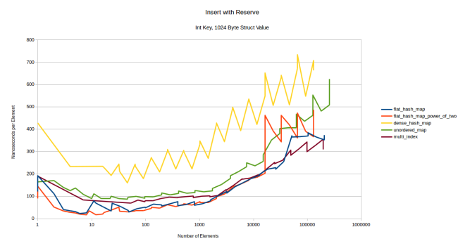
, - boost::multi_index . dense_hash_map , , , - , «» / . , , «» , 1024 ? , .

, : 16 385 . 16 384 . 1028 , , 16 , . , - . , , . , , : , clear_page_c_e . , , clear_page_c_e . - . , .

, . . , .

:

dense_hash_map . , ( Ubuntu 16.04) , .

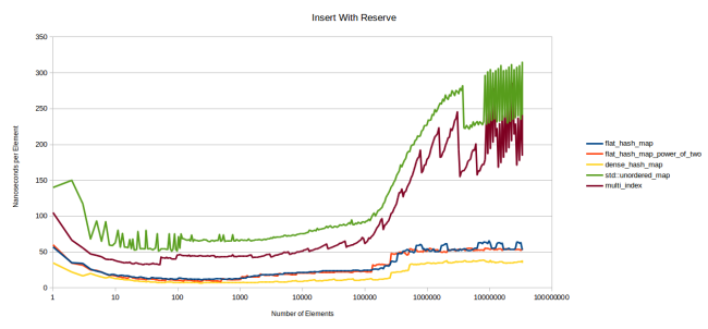
, . . reserve() :

, , . , . : , , - , . - :

dense_hash_map - . . , flat_hash_map_power_of_two 16 385 - clear_page_c_e .

: - , , reserve() . , .

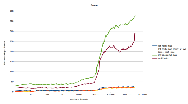
. : 4, 32 1024 . 4- . 32 , . 1024 :

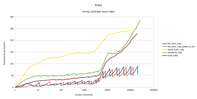
dense_hash_map . : , no-op , dense_hash_map «» /, , 1024 .

: flat_hash_map . , , . , , flat_hash_map , , 1028 .

, . Here is one of them:

1024 , .

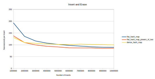
— «, , » . 10 ., 10 . 10 . . - 32 :

flat_hash_map dense_hash_map . .

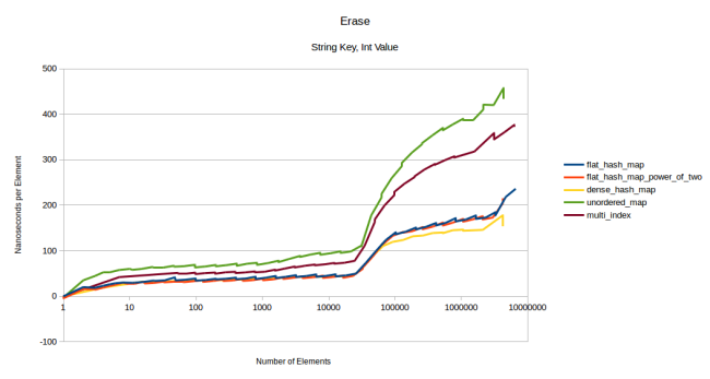
- dense_hash_map . , . , reserve() , . flat- , — . , unordered_map - , , multi_index . , multi_index :

, , 1028 . , : . , , multi_index :

. 32- - . - 1024 , , , , .

, , - . , . . : , , , . . , , :

• , .
• . .
• , , . flat-. flat- .
• , . - .
• google::dense_hash_map .
• boost::multi_index — -. .
• , - , , -, .

Exceptions

, , -, (equality function) . (move constructor) . , . , .

Github . Boost-. ska::flat_hash_map ska::flat_hash_set . , std::unordered_map std::unordered_set .

, . , ska::power_of_two_hash_policy.

, max_load_factor 0,5. 0,9. , . , 70 %, . , max_load_factor , .

Total

, -. . — . log2(n), O(log(n)) O(n). . Robin Hood .

- Boost- hash_map hash_set. !