Z-order vs R-tree, optimization and 3D

Earlier ( 1 , 2 ) we substantiated and demonstrated the possibility of the existence
spatial index, which has all the advantages of the usual B-Tree index and
not inferior in performance index based on R-Tree.
Under the cut, a generalization of the algorithm to three-dimensional space, optimization and benchmarks.

3D

Why do you need this 3D? The fact is that we live in a three-dimensional world. Therefore, the data are presented either in geo-coordinates (latitude, longitude) and then distorted all the more, the further they are from the equator. Or a projection is attached to them, which is adequate only on a certain space of these coordinates. Three-dimensional index allows you to place points on a sphere and thus avoid significant distortion. To obtain a search extent, it suffices to determine the center of the desired cube on the sphere and retreat to the sides in all coordinates by radius.

In principle, the three-dimensional version of the algorithm does not differ from the two-dimensional one — the only difference is in working with the key:

• The alternation of discharges in the key now goes in steps of 3 and not 2; ... z1y1x1z0y0x0
• The key is now 96, not 64 bits. The option to place everything in a 64-bit key is rejected because gives a total of 21 digits per coordinate, which would make us a bit constrained. In addition, 4 and 6 dimensional keys are coming (guess why), and there 64 is not enough, so why delay the inevitable. Fortunately, it is not so difficult
• therefore, the key is no longer bigint, but numeric and in the key interface, methods for translating from numeric and back will be required
• methods of getting the key from the coordinates and back will change
• as well as the method of splitting the subquery. Recall, for splitting a query, which is represented by two keys, corresponding to the lower left and upper right corners of it:
  • found in them the most senior bit different m
  • the upper right corner of the smaller new subquery is obtained by setting all the bits in 1 corresponding to the m coordinate under m
  • the lower left corner of the larger new subquery is obtained by setting all the bits to 0 corresponding to the m coordinate under m
  Actually, nothing has changed, just the digits of one coordinate go with another step
  

Numeric

Numeric itself is not directly accessible to us from the extension. It is necessary to use the universal function call mechanism with marshalling - DirectFunctionCall [X] from 'include / fmgr.h', where X is the number of arguments.

Inside numeric is arranged as an array of short, each of which contains 4 decimal digits - from 0 to 9999. There are no shifts or divisions with the return of the module in its interface. As well as special functions for working with powers of 2 (with such a device, they are out of place). Therefore, to parse numeric into two int64, you have to act like this:

void bit3Key_fromLong(bitKey_t *pk, Datum dt) { Datum divisor_numeric; Datum divisor_int64; Datum low_result; Datum upper_result; divisor_int64 = Int64GetDatum((int64) (1ULL << 48)); divisor_numeric = DirectFunctionCall1(int8_numeric, divisor_int64); low_result = DirectFunctionCall2(numeric_mod, dt, divisor_numeric); upper_result = DirectFunctionCall2(numeric_div_trunc, dt, divisor_numeric); pk->vals_[0] = DatumGetInt64(DirectFunctionCall1(numeric_int8, low_result)); pk->vals_[1] = DatumGetInt64(DirectFunctionCall1(numeric_int8, upper_result)); pk->vals_[0] |= (pk->vals_[1] & 0xffff) << 48; pk->vals_[1] >>= 16; } 

And for the inverse transformation - like this:

 Datum bit3Key_toLong(const bitKey_t *pk) { uint64 lo = pk->vals_[0] & 0xffffffffffff; uint64 hi = (pk->vals_[0] >> 48) | (pk->vals_[1] << 16); uint64 mul = 1ULL << 48; Datum low_result = DirectFunctionCall1(int8_numeric, Int64GetDatum(lo)); Datum upper_result = DirectFunctionCall1(int8_numeric, Int64GetDatum(hi)); Datum mul_result = DirectFunctionCall1(int8_numeric, Int64GetDatum(mul)); Datum nm = DirectFunctionCall2(numeric_mul, mul_result, upper_result); return DirectFunctionCall2(numeric_add, nm, low_result); } 

Working with arbitrary precision arithmetic is generally not a quick thing, especially when it comes to divisions. Therefore, the author had an overwhelming desire to 'hack' numeric and disassemble it on his own. I had to duplicate the locally definitions from numeric.c and process the raw short'y. It was easy and sped up work dozens of times.
')

Solid subqueries.

As we remember, the algorithm splits the subqueries until the data under it completely fits on one disk page. It happens like this:

1. at the input is a subquery, it has a range of values ​​between the lower left (middle) and upper right (far) corners. Coordinate has become more, but the essence is the same
2. do a search in btree for a key smaller angle
3. get to the leaf page and check its last value
4. if the last value is> = key values ​​of a larger angle, we look through the whole page and enter into output everything that got into the search extent
5. if less, we continue to split the query

However, it may happen that a subquery whose data is contained on dozens or hundreds of pages is completely located inside the original search extent. There is no point in cutting it further; data from the interval can be safely entered into the result without any checks.

How to recognize such a subquery? Pretty simple -

• its size in all coordinates must be degrees 2 and equal (cube)
• the angles must lie on the corresponding grating in increments of the same degree 2

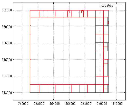
This is what the subquery map looks like before cube optimization:


And so after:

Benchmark

The table summarizes the comparative results of the original algorithm, its optimized version and the GiST R-Tree.
R-Tree is two-dimensional; for comparison, pseudo-3D data was entered into the z-index, i.e. (x, 0, z). From the point of view of the algorithm, there is no difference, we just give the R-tree a certain head start.

The data is 100 000 000 random points in [0 ... 1 000 000, 0 ... 0, 0 ... 1 000 000].

The measurements were conducted on a modest virtual machine with two cores and 4 GB of RAM, so the times have no absolute value, but the numbers of the read pages can still be trusted.
The times are shown on the second runs, on the heated server and the virtual machine. The number of buffers read is on a freshly raised server.

Npoints	Nreq	Type	Time (ms)	Reads	Hits
one	100,000	old new rtree	.37 .36 .38	1.13154 1.13307 1.83092	3.90815 3.89143 3.84164
ten	100,000	old new rtree	.40 .38 .46	1.55 1.57692 2.73515	8.26421 7.96261 4.35017
100	100,000	old new rtree (*)	.63 .48 .50 ... 7.1	3.16749 3.30305 6.2594	45.598 31.0239 4.9118
1,000	100,000	old new rtree (*)	2.7 1.2 1.1 ... 16	07.0775 13.0646 24.38	381.854 165.853 7.89025
10,000	10,000	old new rtree (*)	22.3 5.5 4.2 ... 135	59.1605 65.1069 150.579	3606.73 651.405 27.2181
100,000	10,000	old new rtree (*)	199 53.3 35 ... 1200	430.012 442.628 1243.64	34835.1 2198.11 186.457
1,000,000	1,000	old new rtree (*)	2550 390 300 ... 10,000	3523.11 3629.49 11394	322776 6792.26 3175.36

Where
Npoints - the average number of points in the output
Nreq - the number of requests in the series
Type - 'old' - the original version
'new' - with numeric optimization and solid subqueries;
'rtree'- gist only 2D rtree,
(*) - in order to compare the search time,
I had to reduce the series by 10 times,
otherwise the pages did not fit into the cache
Time (ms) - the average query time
Reads - the average number of reads per request
Hits - the number of calls to buffers
In the form of graphs, these data look like this:

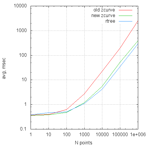
Average request execution time by request size


Average number of reads per request by request size


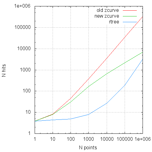
The average number of hits to the page cache per request from the size of the request

findings

So far so good. We continue to move in the direction of use for spatial indexation of the Hilbert curve, as well as full-fledged measurements on non-synthetic data.

PS: the described changes are available here .