Simple Python program for hyperbolic approximation of statistical data

Why do you need it

The laws of Zipf describe the patterns of frequency distribution of words in the text in any natural language [1]. These laws, apart from linguistics, are also applied in economics [2]. To approximate statistical data for objects that obey the Zipf Laws, a hyperbolic function of the form is used:

(one)

where: ab - constant coefficients: x - statistical data of the function argument (as a list): y - approximation of the function values ​​to the real data obtained by the least squares method [3].
')
Usually, for approximating a hyperbolic function using the logarithm method, it is linearized, and then the coefficients a, b are determined and the inverse transform is done [4]. The direct and inverse transformations lead to an additional approximation error. Therefore, I present a simple program in Python, for the classical implementation of the method of least squares.

Algorithm

The source data is given in two lists. where n is the amount of data in the lists.

Get the function to determine the coefficients

The coefficients a, b can be found from the following system of equations: (3)

The solution of such a system is not difficult:

(four),
(five).

Mean approximation error according to the formula: (6)

Python code

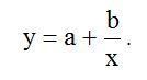
#!/usr/bin/python # -*- coding: utf-8 -* import matplotlib.pyplot as plt import matplotlib as mpl mpl.rcParams['font.family'] = 'fantasy' def mnkGP(x,y): #       n=len(x) #     s=sum(y) #   y s1=sum([1/x[i] for i in range(0,n)]) #  1/x s2=sum([(1/x[i])**2 for i in range(0,n)]) #  (1/x)**2 s3=sum([y[i]/x[i] for i in range(0,n)]) #  y/xa= round((s*s2-s1*s3)/(n*s2-s1**2),3) #       b=round((n*s3-s1*s)/(n*s2-s1**2),3)#  b     s4=[a+b/x[i] for i in range(0,n)] #     so=round(sum([abs(y[i] -s4[i]) for i in range(0,n)])/(n*sum(y))*100,3) #    plt.title('  Y='+str(a)+'+'+str(b)+'/x\n  --'+str(so)+'%',size=14) plt.xlabel(' X', size=14) plt.ylabel(' Y', size=14) plt.plot(x, y, color='r', linestyle=' ', marker='o', label='Data(x,y)') plt.plot(x, s4, color='g', linewidth=2, label='Data(x,f(x)=a+b/x') plt.legend(loc='best') plt.grid(True) plt.show() x=[10, 14, 18, 22, 26, 30, 34, 38, 42, 46, 50, 54, 58, 62, 66, 70, 74, 78, 82, 86] y=[0.1, 0.0714, 0.0556, 0.0455, 0.0385, 0.0333, 0.0294, 0.0263, 0.0238, 0.0217, 0.02, 0.0185, 0.0172, 0.0161, 0.0152, 0.0143, 0.0135, 0.0128, 0.0122, 0.0116] #      y=1/x mnkGP(x,y) 

Result

We took data from the equilateral hyperbola function, so we got a = 0, b = 10 and an absolute error of 0.004%. So the function mnkGP (x, y) works correctly and can be inserted into the application program.

Approximation for power functions

For this, Python has a scipy module, but it does not support the negative degree d of the polynomial. Consider the implementation code for the approximation of data by a polynomial.

 #!/usr/bin/python # coding: utf8 import scipy as sp import matplotlib.pyplot as plt def mnkGP(x,y): d=2 #   fp, residuals, rank, sv, rcond = sp.polyfit(x, y, d, full=True) #  f = sp.poly1d(fp) #   print(' -- a %s '%round(fp[0],4)) print('-- b %s '%round(fp[1],4)) print(' -- c %s '%round(fp[2],4)) y1=[fp[0]*x[i]**2+fp[1]*x[i]+fp[2] for i in range(0,len(x))] #   a*x**2+b*x+c so=round(sum([abs(y[i]-y1[i]) for i in range(0,len(x))])/(len(x)*sum(y))*100,4) #   print('Average quadratic deviation '+str(so)) fx = sp.linspace(x[0], x[-1] + 1, len(x)) #    len(x)     plt.plot(x, y, 'o', label='Original data', markersize=10) plt.plot(fx, f(fx), linewidth=2) plt.grid(True) plt.show() x=[10, 14, 18, 22, 26, 30, 34, 38, 42, 46, 50, 54, 58, 62, 66, 70, 74, 78, 82, 86] y=[0.1, 0.0714, 0.0556, 0.0455, 0.0385, 0.0333, 0.0294, 0.0263, 0.0238, 0.0217, 0.02, 0.0185, 0.0172, 0.0161, 0.0152, 0.0143, 0.0135, 0.0128, 0.0122, 0.0116] #      y=1/x mnkGP(x,y) 

Result

As follows from the graph, when the parabola approximates the data varying in hyperbola, the average error increases, and the free term of the quadratic equation vanishes.

The resulting functions will be used to analyze the laws of Zipf (Zipf), but this will be done in the next article.

References:

1. The laws of Zipf (Zipf) tpl-it.wikispaces.com/ Laws + Zipf +%28 Zipf % 29
2. Zipf's law is. dic.academic.ru/dic.nsf/ruwiki/24105
3. The laws of Zipf. wiki.webimho.ru/zak- zipf
4. Lecture 5. Approximation of functions by the method of least squares. mvm-math.narod.ru/Lec_PM5.pdf
5. Average approximation error. math.semestr.ru/corel/zadacha.php