What is logic programming and why do we need it
The one who in childhood did not write on the Prologue has no heart, and the one who writes on it today has no brains. ( original )
If you are always tormented by agonizing doubts - what the hell is Logical Programming (LP) and, in general, why is it necessary? This is an article for you.
You can divide programming languages into groups in different ways (they are often called programming paradigms), for example, like this:
- structural : the program is divided into blocks - subroutines (isolated from each other), and the main controls are the sequence of commands, branching and loop.
- object-oriented : the task is modeled as objects that send messages to each other. Objects have properties and methods. Abstraction. Encapsulation. Polymorphism. Well, in general, everyone knows.
- functional : the base element is a function and the task itself is modeled as a function, and, more precisely, most often as a composition, if f (.) and g (.) are functions, then f (g (.)) is their composition.
- logical : here, as a rule, the extravaganza begins - if hundreds of articles, books, reviews, presentations and textbooks are written about the first three, here we can see at best something about Prolog and the development of Pink Floyd and Procol Harum (at least they were lucky with the music then) and this is where the story ends.
Here I am going to correct this mistake.
The most important thesis of this article:
Logical programming! = Prolog.
In general, the last one you probably do not need. But the first may well be.
The structure of the article :
- What is the prologue and why you probably do not need it
- Why it is needed, or a brief introduction to Answer Set Programming
- We solve problems on ASP
- Combinatorial optimization
- Probabilistic LP: ProbLog
- LP on classical logic FO (.) And IDP
- Sketched Answer Set Programming
- Experimental analysis
- Testing and correctness of programs
- Conclusion
This article is (possibly) for the first time in Russian, the main aspects of modern logic programming are gathered together with an explanation of why they are needed. Logical programming (LP) is directly related to the topic of my PhD (there will be a separate detailed post about it). In the course of work, I noticed that the material in Russian practically does not exist and decided to fill this gap (there is not even an ASP article in the Russian Wikipedia that would be worth writing).
Parts of the article may not be directly related to each other, such as Sketching and Problog - in a sense, this is a personal review of the most interesting topics and developments in the field of logic programming. It will certainly not be possible to cover all the topics related to the LP - but we can assume that this is the first step for the interested reader to dive into the topic or imagine that the LP is such a beast.
What is the prologue and why you probably do not need it
Prolog (Programming in Logic, original: programmation en logique) was developed in Marseille in the early 70s by Alain Colmereau. The basis of the language is the procedural interpretation of Horn's logical expressions (that is, how exactly one can machine execute) statements of the form:
a :- b, c, d,...,z. What can be read as: "if the conditions b, c, d, ..., z are satisfied, then" a "must be true.
And, simply speaking (here we omit all the technical details), it can be rewritten in the form of logical following:
In fact, Sir Bob Kowalski - came up with such a thing: the statement "a" is true if we prove that all the prerequisites for it are true. (By the way, an excellent and cheerful man - still healthy and pouring jokes and tales, a year ago at a conference in the Royal Community in London, he gave an excellent and at times ridiculous lecture on the history of Prolog and logical programming.)
What is salt, Kowalski? If we take the expression "a: - b, c, d", then it can be read as follows:
"a" is true if I can: prove "b", prove "c" and prove "d".
Then each program is a set of theorems for the derivation of assertions, and each expression is “proved” (an attentive reader will of course notice the Curry-Howard isomorphism here).
The task becomes a little more fun if you add a negative here. In Prolog, it is called negation as failure and differs from classical negation in logic. In theory, it sounds like this: if I could not prove the assertion "a", then it is false. In logic, this assumption is called closed world assumption, and sometimes it is very meaningful.
Negation as Failure and Closed World Assumption
Imagine a bus schedule for route 11 of the city of Samara, fragment:
- 15:15
- 3:45 pm
- 16:15
- 4:45 pm
- 17:15
Question: Is there a bus at 16:00? It is not there, because we cannot prove that it is according to the schedule - i.e. the schedule has a complete picture of the world of the 11th route in the city of Samara. Hence the name “closed world assumption” - the assumption that the entire conditional world is described by this program - everything is out of it - false. As a rule, it is also used in databases - by the way I wrote about them here .
Prologue as Turing is a complete programming language
Together with a couple more interesting operators (such as cut) from the Prologue it turns out - Turing full language - in short - if the program on the prolog P computes the function f (x), then there is a program M in any other Turing full language that also computes f (x ). Thus, if you can solve a program in Prolog, it means you can write a solution in any other language (Python, Java, C, Haskell, etc). No chakras open here.
In general, the solution of the problem on the Prologue is decomposed according to Bob Kowalski into the scheme
Algorithm = Logic + Control
A good example of a problem that is well formulated and solved on a prolog is a set of rules according to which a certain condition is fulfilled or not. However, you yourself will have to specify a solution search algorithm — what is the space of allowable values, in what order do they cost, and so on. In essence, you are modeling a problem in the form of inference rules and using inference rules you define a solution search procedure (order of rules, cut, transition from values in the list from rule to head body, etc.) and admissible solution space.
Let's take as an example a quick sort on the prologue - my comments, the code from The Art Of Prolog (if you have a spontaneous desire read rap to study the Prologue, I recommend this particular book)
quicksort([X|Xs],Ys) :- % head: X -- pivot element, Xs -- the rest, Ys -- sorted array partition(Xs,X,Littles,Bigs), % X divides Xs into Littles = [x < X for x in Xs], and Bigs quicksort(Littles,Ls), % The smaller ones are sorted into Ls quicksort(Bigs,Bs), % Same for biggies append(Ls,[X|Bs],Ys). % Then Ys -- output is literally Ls + [X] + Bs quicksort([],[]). % empty array is always sorted partition([X|Xs],Y,[X|Ls],Bs) :- X =< Y, partition(Xs,Y,Ls,Bs). % If X an element of the given array is above Y, it goes into biggies partition([X|Xs],Y,Ls,[X|Bs]) :- X > Y, partition(Xs,Y,Ls,Bs). % else into littles partition([],Y,[],[]). % empty one is always partitioned We see that the quicksort predicate is defined for two cases - an empty and non-empty list. We are interested in a non-empty case: there is a list [X | Xs] in it, where X is the head of the list, that is, the first element (car is for those who think that there are few brackets in this program) and Xs is the tail (tail, aka cdr) is split into two Bigs and Littles lists - those who are bigger and those who are smaller, X. Then both of these lists are recursively sorted and combined into the final output list Ys. As we see in general, we set the output rules for the operation of the entire algorithm.
What is good prologue? He is good with formal semantics - i.e. you can formally show properties (for example, prove that the program is higher and actually sorts numbers), extends well into a probabilistic case (see the section ProbLog) and generally expands well, is a convenient language for modeling logical problems, well suited for mathematical works, for meta-linguistic operations and so on.
In short, if you don’t write a scientific paper, where you need to formally show the behavioral properties of a program, you probably don’t really need a Prolog. But maybe logic programming will be useful to you?
Why it is needed, or a brief introduction to Answer Set Programming (ASP)
A brief explanation of what an ASP is:
if SAT is assembler, then modern ASP is C ++.
Here it is worth starting with such a thing as declarative programming and the principle of resistance to change ( elaboration tolerance principle ) by John McCarthy (who invented LISP, influenced Algol and generally proposed the term "Artificial Intelligence").
What is a declarative approach? In short, we describe the problem and its properties, and not how to solve it. In this case, the task is most often represented as:
Problem = Model + Search
Where do we regularly meet with this approach? For example, in SQL databases, this is a declarative query language, and the DBMS deals with the search for an answer to this query. Thousands of efficient algorithms have been invented for effective DBMS operation, data is stored in an optimized form, indexes are everywhere, query optimization methods, and so on.
But most importantly, the user sees the tip of the iceberg: the language of SQL. And having some idea about the DBMS, the user can write effective queries. To begin with, we will explain the principle of resistance to change with a simple example. Suppose that we wrote a simple query Q, which considers the average salary in the departments of the company. After some time, we were asked to slightly change the request - for example, to disregard management in calculations - we were interested in the average salary of technical specialists. In this case, you only need to add the condition "role! = 'Manager'" to the Q query.
This means that our new Q_updated request is represented as a basic request + an additional condition. Speaking a little more generally, we see that
Variation of Tasks = Basic Model + Additional Condition
This means that when we slightly change the condition of the problem to some additional condition X, we need to change the model (which models the original problem in some formal language, for example, SQL), adding the additional condition C_X.
And here is ASP and Logic Programming?
References:
- A lot of material can be found on the page of Professor Torsten Schaub.
- Stephan Halbobbler's Tutorial
- Compilation video tutorial: into into ASP , ASP for Knowledge Representation
- Good intro from Thomas Eiter: ASP primer
- ASP in Practice book - used to be freely available (I don’t see a direct link now)
What is the fundamental difference between Prolog and ASP? As a matter of fact, ASP is a declarative constraint language, i.e., we define a search space in the form of special constraints called choice rules, for example:
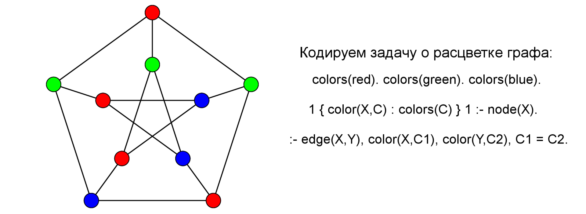
1 { color(X,C) : colors(C) } 1 :- node(X). Such rules define the search space - literally reads like this: for each X in the predicate (read here - in the set) node, ie, for each vertex X - one must be true - the one to the left of "{" and only one - one to the right of "}" atom color (X, C), such that C comes to us from a variety of colors (unary predicate colors / 1).
One of the main features of ASP is that the constraints define what is NOT a solution, for example, consider the following rule:
:- edge(X,Y), color(X,Cx), color(Y,Cy), Cx = Cy. Restrictions (in the scientific English-language literature the term is used: integrity constraints ) - in fact, the rules from the very beginning of the article - only they have an “empty head” ~ empty head: and in fact, this is an abbreviation of the rules of the form:
false :- a_1, a_2, … a_n those. if a_1, ... a_n are executed, then “false” is output and this is not a model.
(more precisely: false is the syntactic construction for b: - a_1, .... a_n, not b. - b is inferred under the assumption that b is wrong - which is a contradiction).
This concludes the theoretical insight and take a closer look at the rule - it states the following: if there is an arc between X and Y, color X is Cx, and color Y is Cy and Cx == Cy, then this is NOT a solution.
By the way, people familiar with ASP would probably have written this rule like this:
:- edge(X,Y), color(X,C), color(Y,C). Variables with the same name within the same rule are considered equal (and most likely it will help at the grounding stage - but this is a separate story).
Let us proceed to the description of the entire task as a whole (and a couple more).
Parse a couple of popular combinatorial problems: NP-complete and not-so
The code described here is best run in Clasp (where it was tested and tested before artistic processing and writing of comments).
We will talk about the following tasks:
- coloring of the graph : given the graph, it is necessary to determine whether it is possible to color it in three colors so that no two vertices are painted in the same color
- black and white queens : on the board n by n, arrange the k black and white queens, so that no two queens of different colors should beat each other
And we will solve each of them with the help of ASP, and at the same time we will analyze the basic modeling techniques.
Coloring graph
Dan Count:
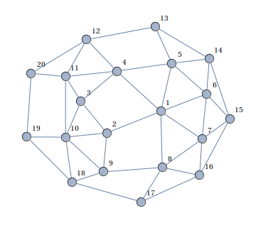
It is necessary to color its vertices in three colors (red-blue-green) so that no two adjacent vertices are the same color, or to say that this is impossible.
Output: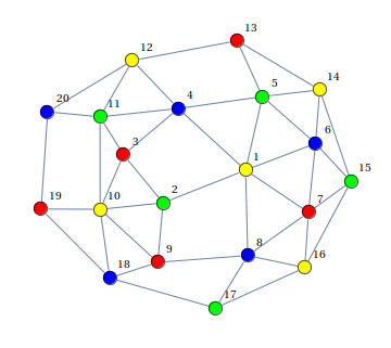
(pictures taken from here )
We have already disassembled the basic constructions of the ASP code - let's go through the remaining elements: node / 1 (node (a). Node (b) ...) - declares a set of vertices of the graph, the order is not important, edge / 2 - announces arcs. Such atoms in ASP (and logical programming) are called facts, in fact, this is an abbreviation of “a: - true.”, And is derived simply from a statement that is always true, that is, atoms define the given data.
% -- , "%" % node(a). node(b). node(c). node(d). % edge(a,b). edge(a,d). edge(b,c). edge(b,d). edge(c,d). % , X Y, , Y X -- edge(Y,X) :- edge(X,Y). % colors(red). colors(green). colors(blue). % , , colors(.) 1 { color(X,C) : colors(C) } 1 :- node(X). % X, Y (- ) , Cx = Cy, :- edge(X,Y), color(X,C), color(Y,C). % #show color/2. Black and white queens
About the arrangement of queens (I include this variation) I wrote earlier in more detail here .
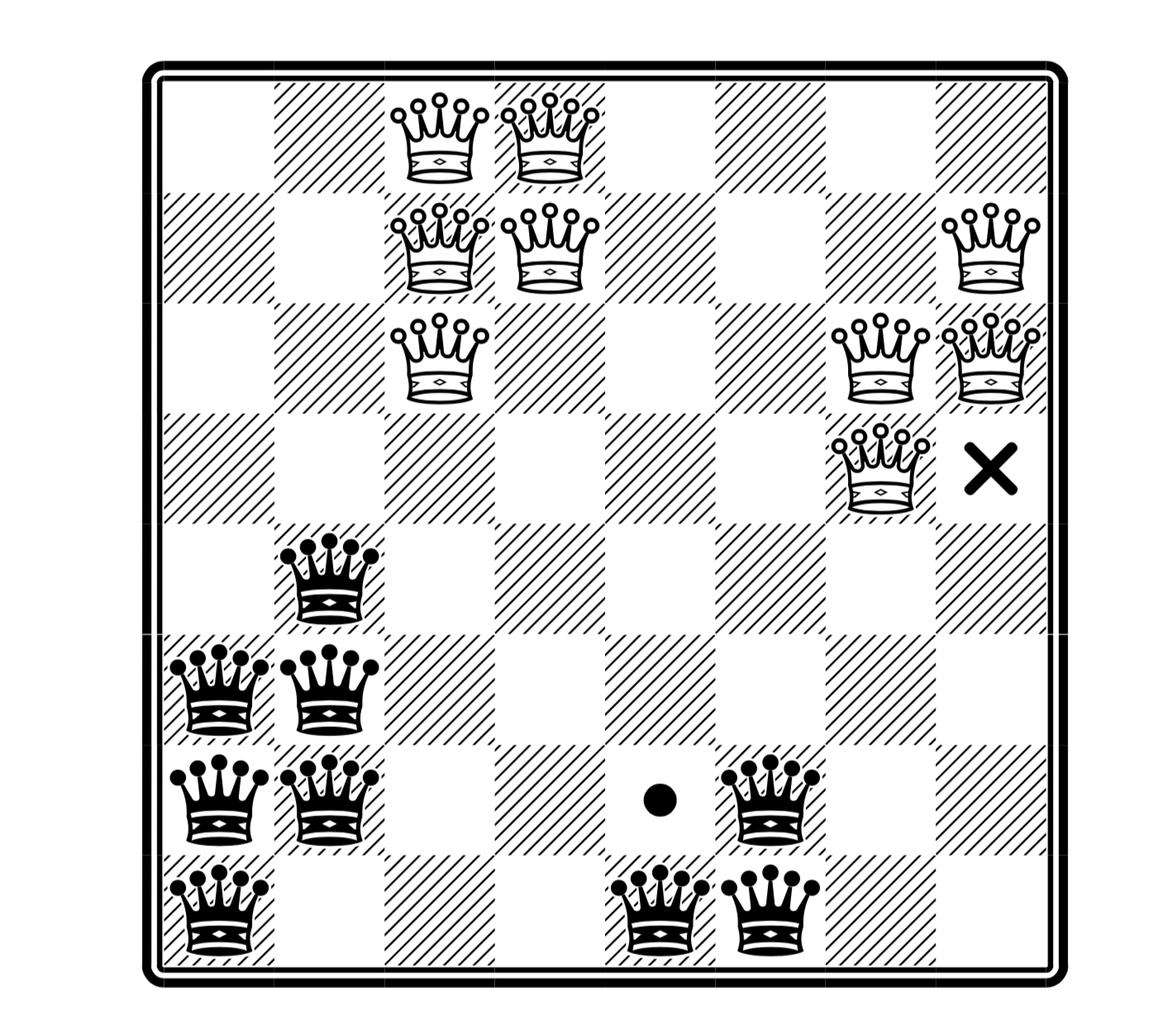
(here is the maximum number of queens, and in the place of the cross you can put white, and in place of the black point - but not both at once; taken from the article )
The code given here solves both a simple polynomial version of the queens arrangement and the NP-full version (see the habr-article about queens; here we assume that the result for the classic version also applies to this variation).
% "k" "m" #const k=2. #const m=4. % color(b). color(w). col(1..m). row(1..m). % k , k { queen(C,Row,Col) : col(Col), row(Row) } k :- color(C). % Rw -- row white, Cb -- column black, etc % :- queen(w,Rw,Cw), queen(b,Rb,Cb), Rw = Rb. % :- queen(w,Rw,Cw), queen(b,Rb,Cb), Cw = Cb. % :- queen(w,Rw,Cw), queen(b,Rb,Cb), | Rw - Rb | = | Cw - Cb |. Let us analyze the code in a little more detail, the following rules set the parameters of the board - in fact, we could solve the problem and with a large number of colors of the queens — the colors are written here as predicate values color/1 .
% "k" "m" #const k=2. #const m=4. % color(b). color(w). col(1..m). row(1..m). Next we need to declare the search space:
% k , k { queen(C,Row,Col) : col(Col), row(Row) } k :- color(C). In essence, this rule reads as follows: for each color C , there must be k and exactly k queens of color C , and the value of Row and Col must be from the set of col/1 and row/1 predicates. Simply put, for each color we set the number of correct (on the board) queens to be k.
Next, we describe what is not a solution: if we are of a different color on one line, column or diagonal:
% :- queen(w,Rw,Cw), queen(b,Rb,Cb), Rw = Rb. % :- queen(w,Rw,Cw), queen(b,Rb,Cb), Cw = Cb. % :- queen(w,Rw,Cw), queen(b,Rb,Cb), | Rw - Rb | = | Cw - Cb |. In essence, we see that our code decomposes well into two parts: search space (guess) + answer validation (check) —as ASP is called the guess-and-check paradigm, and all code goes well with the equation Problem = Data + Model - unlike SAT, if I change the data - I add new queens, then the restrictions themselves (model rules) will not change. In general, we could rewrite these rules so that they even take colors as parameters.
Briefly about combinatorial optimization
The essence is simple: there is a combinatorial problem, such as searching for the Hamilton cycle (NP-complete problem), but there is an additional condition above: something needs to be minimized - for example, the weight of the path (the number of colors for coloring the graph, maximize the number of queens or queens colors, etc.). ) As a rule, this gives a jump in the complexity of the task and makes the search quite complex. ASP has a standard mechanism for solving combinatorial optimization problems.
Let us analyze the Hamilton cycle search problem with weight path optimization (code from the book Answer Set Solving in Practice. Martin Gebser et al .; comments are mine)
% === GUESS === % -- 1 { cycle(X,Y) : edge(X,Y) } 1 :- node(X). % 1 { cycle(X,Y) : edge(X,Y) } 1 :- node(Y). % 1 % === AUXILIARY INFERENCE === reached(Y) :- cycle(1,Y). % reached(Y) :- cycle(X,Y), reached(X). % === CHECK === % - -- :- node(Y), not reached(Y). % === MINIMIZE === % -- , #minimize [ cycle(X,Y) = C : cost(X,Y,C) ]. In essence, we see that the combinatorial optimization problem in ASP is well decomposed into a declarative equation:
Problem Model = Guess + Check + Minimize
Also in the task there is a part of the output of new facts (auxiliary inference), which are then used in constraints. This is also pretty standard for programs written in ASP.
Probabilistic Prolog - ProbLog
Prolog is good because it expands well - as a language, including in a probabilistic case - ProbLog (I read it as a joke always, like Probloch - reference to its Flemish origin and how the authors read it) - Probabilistic Prolog.
The theoretical foundations of probabilistic logic programming are set forth in the article
A Statistical Learning Methods for Logic Programs with Distribution Semantics by Taisuke Sato
(By the way, he was still in a sober mind and sound memory - he spoke at ILP 2015 in Kyoto - where he asked the participants a lot of interesting and insidious questions)
The main materials on the topic can be found here (there is also an online editor and tutorial, articles, etc.)
Essentially imagine that now the rules of the prologue deduce not a fact, but the probability that this fact is true, for example, imagine that we have a set of dishonest coins, dishonest because the probability of an eagle falling out is not 0.5, but for example 0.6. probability of falling eagle, if we throw up four such coins?
% Probabilistic facs: 0.6::heads(C) :- coin(C). % Background information: coin(c1). coin(c2). coin(c3). coin(c4). % Rules: someHeads :- heads(_). % Queries: query(someHeads). In the first rule, we describe what random variables we have - these are variables that describe the eagle falling out (the facts about the coins themselves are deterministic), then we describe the stochastic quantity - someHeads - the loss of at least one eagle, through our probabilistic values - coins. And the last is the query: what is the probability of the eagle falling out?
In fact, ProbLog is a very convenient system for modeling tasks that are represented as a group of rules (for example, a business of logic) with a probabilistic outcome.
Logical programming in classical logic FO (.) And IDP
FO (.) And IDP is in many ways a very similar system with Answer Set Programming: FO (.) - First Order and (.) - reference to extensions of the language in case of inductive definitions, aggregation, and so on. And IDP is a system that supports the FO (.) Language. Here and further, we do not distinguish between them (and in general this difference seems to be significant only for the authors - but there, as the main ideological creator of FO (.) And IDP, Mark Denecker, all five years of my PhD, showed me the difference, I decided to make a difference at least somewhere between them).
In essence, the whole difference is that instead of the rules of inference in the spirit of Prologue, we use classical logic. IDP also supports a simple type system.
/********************************* A Sudoku solver in IDP *********************************/ vocabulary V { type row isa int // The rows of the grid (1 to 9) type column isa int // The columns of the grid (1 to 9) type number isa int // The numbers of the grid (1 to 9) type block isa int // The 9 blocks of 3x3 where the numbers need to be entered liesInBlock(row, column, block) //This declares which cells belongs to which blocks. //This means that liesInBlock(r, k, b) is true if and only if // the cell on row r and column c lies in block b. solution(row, column) : number //The solution: every cell has a number //A cell is represented by its row and column. //For example: solution(4,5) = 9 means that the cell on row 4 and column 5 contains a 9. } theory T : V { //On every row every number is present. ! r : ! n : ? c : solution(r,c) = n. //In every column every number is present. ! c : ! n : ? r : solution(r,c) = n. //In every block every number is present. ! b : ! n : ? rc : liesInBlock(r,c,b) & solution(r,c) = n. //Define which cells lie in which block { liesInBlock(r,k,b) <- b = (((r - 1) - (r - 1)%3) / 3) * 3 + (((k - 1)-(k - 1)%3) / 3) + 1. } } (I would simplify the code and liesInBlock zhardkodil - code from the examples of the editor
, . : . — solution(row, column) -> {1,...,9}, :
, , (r, c) n . .
Sketched Answer Set Programming
— ( , , ). , (logic programming) (machine learning), Inductive Logic Programming . , ASP.
Sketched Answer Set Programming by Sergey Paramonov, Christian Bessiere, Anton Dries, Luc De Raedt
, ASP — Constraint Programming Essense .
-- ASP, :
:- queen(w,Rw,Cw), queen(b,Rb,Cb), Rw != Rb. :- queen(w,Rw,Cw), queen(b,Rb,Cb), Cw != Cb. :- queen(w,Rw,Cw), queen(b,Rb,Cb), |Rw - Rb| != |Cw - Cb|. Unsatisfiable . sketching , " , " , — " , "
[Sketch] :- queen(w,Rw,Cw), queen(b,Rb,Cb), Rw ?= Rb. :- queen(w,Rw,Cw), queen(b,Rb,Cb), Cw ?= Cb. :- queen(w,Rw,Cw), queen(b,Rb,Cb), Rw ?+ Rb ?= Cw ?+ Cb. [Examples] positive: queen(w,1,1). queen(w,2,2). queen(b,3,4). queen(b,4,3). negative: queen(w,1,1). queen(w,2,2). queen(b,3,4). queen(b,4,4). , , , , , . ( ).
, , .
vs
Relational Data Factorization (Paramonov, Sergey; van Leeuwen, Matthijs; De Raedt, Luc: Relational data factorization, Machine Learning, volume 106) , :
— ( + ~= ) — — , ASP — .
: + , :
= + ASP
, structured frequent pattern mining (. Paramonov, Sergey; Stepanova, Daria; Miettinen, Pauli: Hybrid ASP-based Approach to Pattern Mining, Theory and Practice of Logic Programming, 2018 ):
( ; — -, )
, ( )
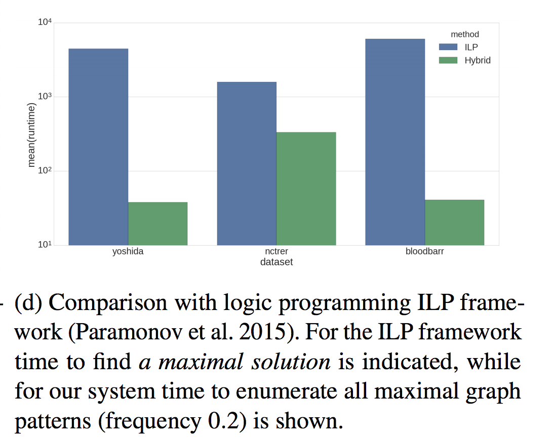
, , .
, , , . :
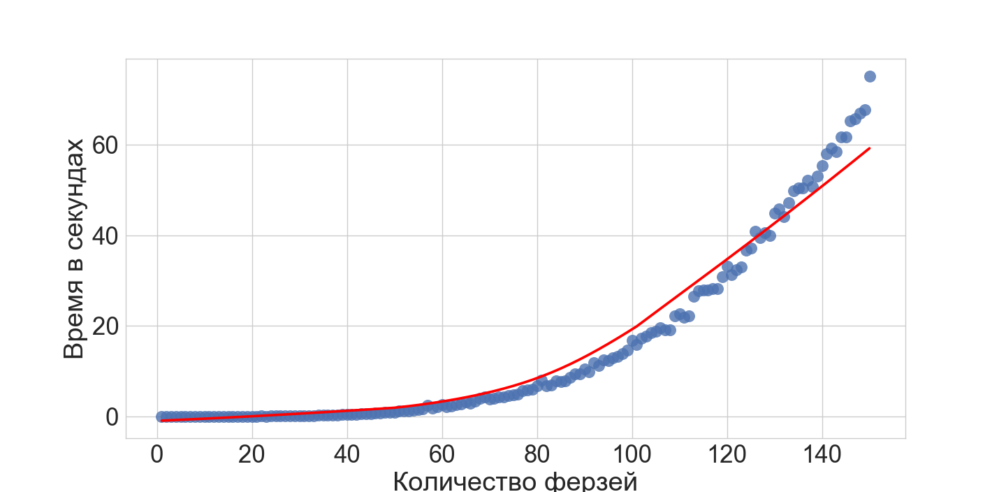
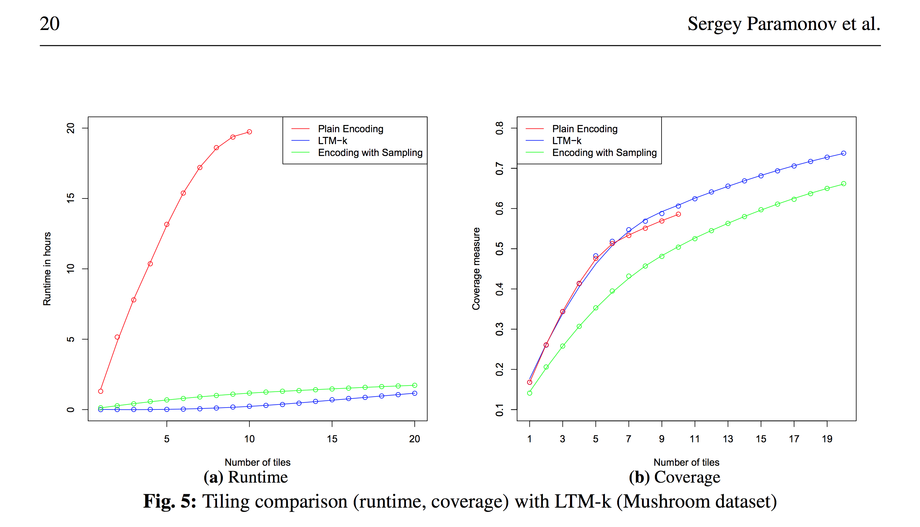
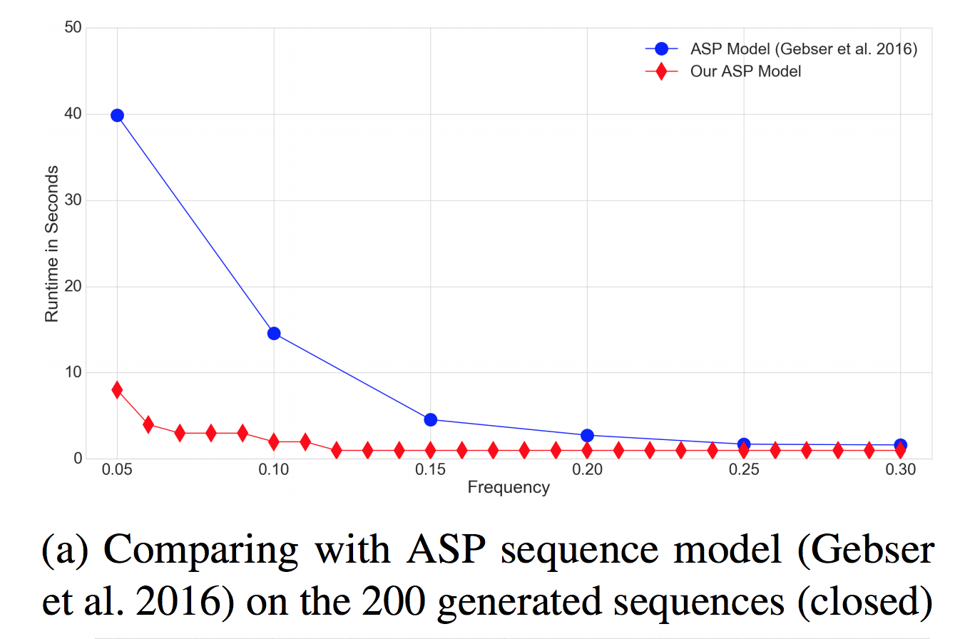
, , , , LCM-k:
, , "ASP solver", .. Answer Set Programming. , — . , , — . , , ASP .
, ( ), "?" :
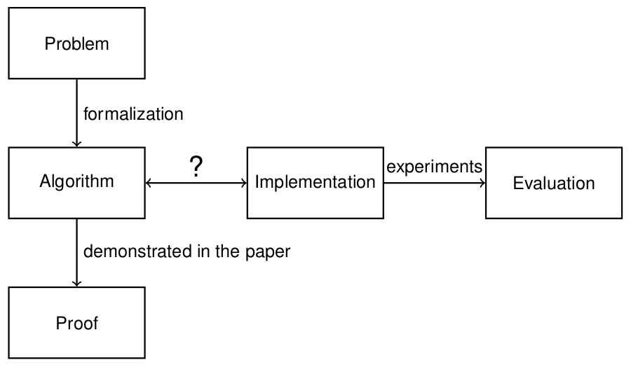
ASP — algorithm implementation ( ASP ), .
, :
- baseline
Conclusion
() — . (tl;dr) :
- != ;
- ASP ;
- : + ;
- ASP : " - ?", " ?", etc;
- , , ASP .
')
Source: https://habr.com/ru/post/322900/
All Articles