Quite often, enterprise data processing tasks involve data accompanied by a time stamp. In R, such labels are usually stored as the POSIXct class. The choice of methods for working with this type of data according to the principle of analogy can lead to a great disappointment and conviction about the extreme slowness of R. Although, if you look at this a little more closely, it turns out that the point is not quite R, but the hands and head.

Below I will touch on a couple of cases that met this month and possible solutions. In the course of the solution, very interesting questions arise. At the same time I will mention the tools that are extremely useful for solving such problems. Practice has shown that few know about their existence.

Case №1. IT system event data processing

From the point of view of business, the “as if” task is trivial. It is necessary to display an event stream of a distributed system in a intelligible form over a certain time period. And then provide a diverse criterial "cutting". The data source is the subsystem logging components of the IT system.

From the standpoint of convenience of perception, the representation in the form of a “heat map” is optimal for a high-level review of such data. Here is an example of the generated graphics.

It makes no sense to reinvent the wheel, the approach described in the article “Bob Rudis, Making Faceted Heatmaps with ggplot2” was used . As a matter of fact, since the data are essentially identical and represent a timestamp with a corresponding set of metrics, then I will appeal to this article and publicly published data in order not to disclose private information.

Nuance number 1

is that there are several sources of events and they are located in different time zones. The time in the source data is measured in UTC, and the analytics must be tied to the work cycle in time of the local time zone. Baseline data is as follows:

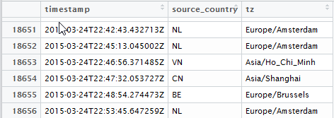
where timestamp is UTC the event time in ISO8601 format in text form, tz is the time zone marker in which this event occurred.

Nuance # 2

This is because the dplyr::do() approach used in the article is obsolete since the release of the purrr package. Photographer 's comment: dplyr :: do () is now basically deprecated in favor of the purrr approach . And this means that the code should be adapted to the modern approach.

Immediately proceed to the purrr , skipping the approaches associated with the for loops and the Vectorize Vectorize as ineffective. Unfortunately, attempts to apply “in the forehead” vectorization to POSIXct value vectors with different timezone is impossible. The answer is the result of a close look at the POSIXct vector of values ​​by the dput function. Timezone is an attribute of a vector, but not a single element!

For this reason, applying the functional approach of the map to the POSIXct variable by the element-wise method gives a disappointing result: on a sample of 20 thousand records, the processing time is almost 20 seconds. At the same time, the vectorization properties of the ymd_hms() function are ymd_hms() , otherwise the result would be even worse.

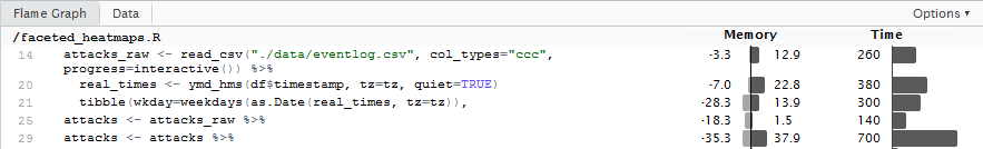
 attacks_raw <- read_csv("./data/eventlog.csv", col_types="ccc", progress=interactive()) %>% slice(1:20000) attacks <- attacks_raw %>% # mutate(rt=map(.$timestamp, ~ ymd_hms(.x, quiet=FALSE))) %>% #    ~  8   mutate(rt=ymd_hms(timestamp, quiet=FALSE)) %>% mutate(hour=as.numeric(map2(.$rt, .$tz, ~ format(.x, "%H", tz=.y)))) %>% mutate(wkday_text=map2(.$rt, .$tz, ~ weekdays(as.Date(.x, tz=.y)))) %>% unnest(rt, hour, wkday_text) 

We are trying to figure out the reason for this behavior. To do this, use the code profiling tool. Interested parties can see the details on the Profvis website: Profvis - Interactive Visualizations for Profiling R Code , as well as see the video:

• 2016 Shiny Developer Conference Videos: Profiling and performance - Winston Chang ;
• rconf2017: Understand Code Performance with the profiler - Winston Chang .

The result of the profiling is as follows:

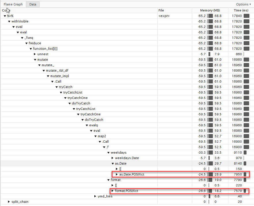
It can be seen that the main time is spent on multiple conversions POSIXct , POSIXlt . There are certain explanations for this, with certain positions can be found here: “Why compared with as.POSIXct?” .
But for us there are several main conclusions:

1. maximally pull out all actions with dates beyond the limits of the function;
2. use vectorization for POSIXct values ​​with the same tz (i.e., we will not be forced to pass time-zone as a parameter);
3. use the features of the lubridate package when, under certain text formats, the conversion of chr->POSIXct is not performed by the basic R functions, but repeatedly optimized (see the fasttime package).
4. instead of dplyr::do use purrr::map2 .

Slightly modifying the code we get the acceleration almost 25 times . (when running on a larger data array, the gain is obtained almost 100 times ).

The code looks like this:

 attacks_raw <- read_csv("./data/eventlog.csv", col_types="ccc", progress=interactive()) %>% slice(1:20000) parseDFDayParts <- function(df, tz) { real_times <- ymd_hms(df$timestamp, tz=tz, quiet=TRUE) tibble(wkday=weekdays(as.Date(real_times, tz=tz)), hour=as.numeric(format(real_times, "%H", tz=tz))) } attacks <- attacks_raw %>% group_by(tz) %>% nest() %>% mutate(res=map2(data, tz, parseDFDayParts)) %>% unnest() 

One of the key "chips" is grouping by time-zone with the subsequent vectorization of processing.

Case №2. Time Sliding Window

A business case is also trivial. There is an array of temporary data characterizing the response time to user actions.

It is necessary to calculate the APDEX index to assess user satisfaction with the application.

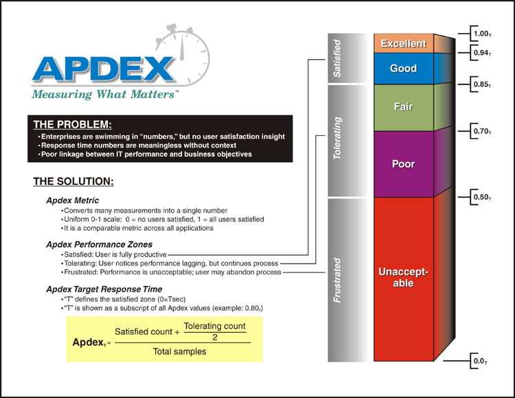
  # ,     3 : # N –     # NS -  ,        [0 – ] # NF –  ,    ( – 4] # (.         4) #  APDEX = (NS + NF/2)/N. 

As a starting point, we use the terrifying results of calculating the metric on a sliding window using the base R. For sampling 2000 records, the calculation time is almost 2 minutes !

 apdexf <- function(respw, T_agreed = 1.2) { which(0 < respw$response_time & respw$response_time < T_agreed) apdex_N <- length(respw$response_time) #APDEX_total apdex_NS <- length(which(respw$response_time < T_agreed)) # APDEX_satisfied apdex_NF <- length(which(T_agreed < respw$response_time & respw$response_time < 4*T_agreed)) # APDEX_tolerated F=4T apdex <- (apdex_NS + apdex_NF/2)/apdex_N return(apdex) } dt = dminutes(15) df.apdex = data.frame(timestamp=numeric(0), apdex=numeric(0)) for(t in seq(from = start_time, by = dt, length.out = floor(as.duration(end_time - start_time)/dt))){ respw <- subset(mydata, t <= timestamp & timestamp < t+dt) df.apdex <- rbind(df.apdex, data.frame(timestamp = t, apdex = apdexf(respw))) } 

We skip all intermediate steps, immediately mark the places for optimization.

1. Transition to functional processing.
2. Carrying out all constant calculations beyond the limits of a function called in a loop. In particular, the status satisfied\tolerated\frustrated is only a function of the response time, but not the measurement time or the calculation window - the takeaway.
3. A crucial point is unproductive copying of objects !!! Despite the fact that data.frame is passed to a function by reference, operations with data.frame inside a function can lead to the creation of a duplicate object, and this is a significant overhead. Optimization of operations using the features of dplyr methods allows minimizing the amount of data copying inside a function, which significantly increases performance. The features of the dplyr methods as well as the means of controlling objects, in particular, the dplyr::changes() function can be found in the article “Data frame performance” Therefore, it is precisely for this reason that a model of individual columns with a response time status is much preferable to a single column with a status type of response time.
4. We carry out the calculation of the range of time windows once at the start of the calculations using the vectorization property. The calculation of the POSIXct + time shift is a very expensive procedure to perform within the loop.
5. We use optimized dplyr functions with external parameterization. This trick allows you to reduce the cost of computation and memory used, but somewhat complicates the syntax by returning from NSE [Non-Standard Evaluation] to SE [Standard Evaluation]. ( filter -> filter_ ). As an introductory information about the SE \ NSE can be found here: "Non-standard evaluation" .

 apdexf2 <- function(df, window_start, cur_time) { t_df <- df %>% filter_(lazyeval::interp(~ timestamp>var, var=as.name("window_start"))) %>% filter_(lazyeval::interp(~ timestamp<=var, var=as.name("cur_time"))) #    ,  summarise s <- sum(t_df$satisfied) t <- sum(t_df$tolerated) f <- sum(t_df$frustrated) (s + t/2)/(s + t + f) } t_agreed <- 0.7 mydata %<>% mutate(satisfied=if_else(t_resp <= t_agreed, 1, 0)) %>% mutate(frustrated=if_else(t_resp > 4*t_agreed, 1, 0)) %>% mutate(tolerated=1-satisfied-frustrated) %>% mutate(window_start=timestamp-minutes(15)) time_df <- mydata %>% select(window_start, timestamp) mydata %<>% select(timestamp, satisfied, tolerated, frustrated) mydata$apdex <- map2(time_df$window_start, time_df$timestamp, ~ apdexf2(mydata, .x, .y)) %>% unlist() 

After a similar optimization, we get a processing time of ~ 3.5 seconds. Acceleration is almost 35 times and is achieved by simply rewriting the code!

But this is not the limit. The above implementation calculates a sliding window for each individual metric. Measurements can come at arbitrary times. But in practice, such accuracy is superfluous, it is quite enough to deduct the calculation of group intervals up to 1-5 minutes. This means that the amount of computation can decrease again by 10, with a proportional reduction in computation time.

In conclusion, I want to note that the current set of packages and tools really allows you to write on R compactly and quickly. In the case when this will not be enough, there is still a reserve in the form of Rcpp - writing separate functions in C ++.

Previous post: “R in enterprise tasks. Tricks and Tricks