PyMC3 - MCMC and not only
PyMC3 - MSMS and not only
![]()
Hi, Habrahabr!
PyMC3 has already been mentioned in this post. There you can read about the basics of MCMC sampling. Here I will tell about the variational conclusion ( ADVI ), about why all this is needed and will show with rather simple examples from the PyMC3 gallery how this can be useful. One such example would be the Bayesian neural network for the classification task, but this is at the very end. Who cares - welcome!
Introduction
Before turning to the main part, I consider it necessary to refresh the terminology of Bayesian analysis. The subject of this subsection of the theory of probability is the derivation of the posterior distribution. The task is as follows:
The analyst wants to learn something about the unobservable (latent) parameters of the model. z and he has some thoughts on how they can be p(z) . In addition, he can judge how well his data D fit into the model with parameters z . This is expressed through credibility p(D|z) - probability of observing the data with the given parameters.
largep(z|D)= fracp(z,D)p(D)= fracp(D|z)p(z)p(D)
Where
p(z) - a priori distribution, assumptions about the expected results.
When you approach the solution of a problem, very often there is an idea of the phenomenon that is being investigated.- For example, take the field of physics. There are laws and mechanisms of interaction, we have a good idea about them (except for some values, such as the coefficient of friction of a substance with a surface). We roughly assume what it should be, based on past experience and accumulated knowledge. At least that it is more than zero. We can build an experiment by creating a physical model with an unknown parameter that we want to evaluate.
- Important note: Sometimes it is tempting to adjust the prior distribution to the observed data. Say, for example, that we figured on the data that the desired z somewhere around 3 and begin to display a posteriori. Wait, but when you, for example, prove a theorem, you do not use its results to prove it? Similarly, the prior distribution should not be based on the data set under study .
- p(D|z) - credibility, assessment of the adequacy of the alleged z . It is expressed in the probability of observing the data subject to the hypothesis chosen z .
- We have the results of the experiment, for each set of parameters we can evaluate, "how well the model describes the world." This idea is used by classic statistics in MLE estimation.
- p(z|D) - a posteriori distribution, the conclusions that we want to get.
- In fact, these are the ideas about the unknown parameters of the model (coefficient of friction) that we formed during the course of the experiment. It can be considered a compromise between old knowledge and new, expressed through p(z) and p(D|z) respectively.
- p(D) - Evidence, the probability of obtaining such data in general, is translated badly into Russian.
Bayesian output
At first glance, nothing special: we have density formulas p(D|z) , p(z) , the density sought is as follows:
largep(z|D)= fracp(D|z)p(z)p(D)= fracp(D|z)p(z) intp(D|z)p(z)dz
Multiply two densities - not a problem. Calculate the integral from below? .. Hmm, well, you can recall the university course of mathematical analysis ... In general, we take, we substitute everything in the formula and it is ready. Armed with this knowledge, you can safely go to explore simple models with simple distributions. However, in more or less approximated examples of life, even such knowledge will not save and it is analytically impossible to take the integral analytically.
Why all this?
Well, if we can not display the distribution p(z|D) why not just restrict ourselves to a point estimate, say, where the distribution density is maximal? Well, or in a pinch, do not even do this and look for a maximum p(D|z) , we want to build a model that explains our data. The first approach is called the MAP (maximum a posterior) score. zmap=argmaxzp(z|D) and the second is ML (maximum likelihood) zml=argmaxzp(D|z) . The second method, almost every student of a technical college was in the course of probability theory.
ML estimates have a number of drawbacks. The most intuitive of them is that even a complex model may seem attractive in terms of this criterion. After all, the more likely the better, but with an increase in parameters, the model can simply repeat the data. This fact is misleading and makes it necessary to justify why the model is adequate. From the point of view of Bayesian inference, you can imagine ML valuation as MAP with p(z)=Uniform[− infty, infty] . Yes, the integral is not taken, but we have a point estimate and this will not interfere with us, we consider the density p(z) constant.
Evidence
largep(z|D)= fracp(z,D)p(D)= fracp(D|z)p(z)p(D) rightarrowmax
large logp(z|D)= log fracp(z,D)p(D)= log fracp(D|z)p(z)p(D) rightarrowmax
large sim logp(D|z)p(z)− logp(D) rightarrowmax
large sim logp(D|z)+ logp(z) rightarrowmax
large sim logp(D|z) rightarrowmax
This kind of prior distribution is called the Improper Priors , and specifically it is also Uninformative (non-informative).
In other words, we have no idea what should be z in fact. Lost the ability to use all available information. For example:
- For some problem from the theory it is reliably known that z strictly greater than zero. This can be corrected by conversion, but if you change the setting to “rather more than less than zero,” then ML cannot take this into account.
- For the case of linear regression, when there are a large number of regressors, there is a belief that not all of them are important. Then in the vector z (coefficients) many zero components.
The standard approach is good simplicity of implementation and the studied asymptotic properties, but MAP is more meaningful in a number of situations.
from theano import theano, tensor as tt import pymc3 as pm import pandas as pd from sklearn import datasets import numpy as np from numpy import random import pylab as plt import seaborn as sns import warnings import scipy.stats as stats warnings.filterwarnings('ignore') %matplotlib inline plt.mpl.style.use('ggplot') Coin example
Let's see what happens with the a posteriori distribution when we get new observations. This is very similar to a change in confidence in its most ordinary sense. At first, we know nothing, but when we get examples, our understanding of unobservable factors changes. For a visual representation, I will use the honest conclusion of the a posteriori distribution.
Having prior Uniform[0,1] (equivalent to Beta[ alpha=1, beta=1] ) for the probability of getting an "eagle" r and having the observation "eagle" t and "tails" f , Total N observations, we obtain the posterior distribution on the probability Beta[ alpha=t+1, beta=f+1] .
largep(r|T=t,F=f)= fracp(T=t,F=f|r)p(r) intp(T=t,F=f|r)p(r)dr
large= fracCkNrt(1−r)f int10CkNrt(1−r)fdf= fracrt(1−r)fB(t+1,f+1)
large=Beta(r| alpha=t+1, beta=f+1)
For visual illustration, several auxiliary functions and synthetic data are required.
# def posterior(t, f): """ t : f : """ return stats.beta(a=t+1, b=f+1) # def plot_pdf(dist, ax, c): space = np.linspace(0, 1) pdf = dist.pdf(space) ax.plot(space, pdf, c=c, alpha=.5) return ax # true_p = .3 # "" random.seed(42) # trials = np.random.uniform(size=100) < true_p # , 1 # [t, f] observed = np.array(list(zip(np.cumsum(trials), np.arange(1, trials.size+1) - np.cumsum(trials)))) observed[:6] array([[0, 1], [0, 2], [0, 3], [0, 4], [1, 4], [2, 4]]) fig, ax = plt.subplots(figsize=(15, 5)) cmap = plt.get_cmap('cool') plot_pdf(posterior(0, 0), ax, cmap(0)) for (t, f), c in zip(observed, np.linspace(0, 1, num=observed.shape[0])): plot_pdf(posterior(t, f), ax, cmap(c)) plt.title(' ') plt.show() 
The more examples we see, the more narrow the posterior distribution becomes, this is a manifestation of confidence in new knowledge. What is more interesting is the behavior of the distribution with a small number of observations: it adequately reflects the uncertainty. This does not happen if we use the methods of classical statistics and look for the MLE estimate. We would get a probability of 0 for an eagle with a small number of observations, which, of course, is not so.
Motivation
PyMC3 allows you to display a posteriori distribution without directly outputting formulas. This makes possible the Bayesian probabilistic inference on virtually any adequate models. Moreover, it can be used to build probabilistic neural networks in which, instead of parameters, distributions and, therefore, predictions are also distributions.
Getting started with PyMC3
The PyMC3 library is written on top of Theano and therefore can be used with it. Theano is a library for tensor algebra and is widely used for deep learning. It supports symbolic operations and differentiation, which makes possible not only the training of neural networks with the help of backprop , but also the Baes variational conclusion.
Working with PyMC3 mostly resembles working with Theano , in one of our previous posts it is well written.
The base part of the library is the model ( pm.Model ), it allows on the fly to make up the a posteriori density (more precisely, its non-normalized part). In order for this to work with a nice interface, a little magic is applied with the context manager. Latent variables in PyMC3 are declared inside the context with model: ...
The latent variables themselves are variables in the sense of Theano , for them everything that is true of ordinary tensors in Theano is true. This is useful to remember, so as not to be afraid to experiment and build more complex models.
We will build the model sequentially in order to demonstrate by an illustrative example that MCMC methods with an increase in the complexity of the model can worsen their results, or, at least, become unacceptably slow.
You can pm.sample it using the pm.sample helper function, it works well with the default settings, but they have been changed for demonstration purposes. By default, suitable parameters are pre-selected for the MCMC method, which is not needed right now.
# import pymc3 as pm with pm.Model() as simple_model: # # norm = pm.Normal('norm', 0, 1) # MCMC NUTS step = pm.NUTS() trace = pm.sample(1000, step=step) # : WARNING (theano.tensor.blas): We did not found a dynamic library into the library_dir of the library we use for blas. If you use ATLAS, make sure to compile it with dynamics library. 100%|██████████| 1000/1000 [00:00<00:00, 1368.27it/s] Trace plot
To visualize the results there are great utilities. For example, TracePlot . This is a graph of the history of the Markov chain. Analyzing it, you can understand how well the algorithm worked and whether it requires additional configuration. Visual quality criteria are:
- Stationarity. Samples must form noise around a value.
- Do not have a strong autocorrelation. Sometimes this can be expected (see below), but it is better that it is not
- All history cannot be from the same recurring point. If some variable remained constant, then most likely something went wrong in the code of the model itself.
pm.traceplot(trace); 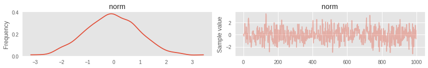
Let's complicate the model a bit
with pm.Model() as simple_model: norm = pm.Normal('norm', 0, 1) # laplace = pm.Laplace('lap', mu=norm, b=3) step = pm.NUTS() trace = pm.sample(1000, step=step) 100%|██████████| 1000/1000 [00:36<00:00, 27.10it/s] Turbulence in the Markov chain for normal distribution became noticeable.
pm.traceplot(trace); 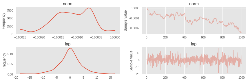
This is what happens when the model becomes non-trivial, although it should have been with an independent normally distributed first variable. For such cases, you can first tighten the ADVI and use the covariance matrix and the means from there to initialize NUTS. But first, more about ADVI.
ADVI
ADVI stands for Automatic Differentiation Variational Inference ( link to the article ). This is perhaps one of the most simple and frequently used algorithms for approximate Bayesian inference. When the dimension of the latent space grows, MCMC methods become either quite complicated to set up (default parameters are not suitable), or the iterations take a huge amount of time. The fact that the default parameters may not be suitable, we have seen above. And then it becomes necessary to at least bring closer the target distribution of those with which we can work.
Theory
The essence of the method is that it approximates the posterior distribution p(z|D) other distribution q(z) , for which we can count the density and sample. In the classical formulation, such a distribution is a multidimensional normal with a diagonal covariance matrix. mathcalN( bar0,diag( bar sigma2)) . This is its main drawback: it is assumed that latent variables are independent, but this, of course, is not always the case. Nevertheless, even with such a strong premise one can achieve good results. Next, we will see how this simplification saves computational resources.
Formulation of the problem
Let there be observations mathcalD , parametric model with parameters z in mathcalRn and its likelihood function p(D|z) . In addition, the Bayesian approach requires an a priori distribution on the model parameters. p(z) . By Bayes' rule, we derive the posterior distribution of the parameters:
largep(z|D)= fracp(D|z)p(z) intp(D|z)p(z)dz
A part without a normalizing constant is usually not difficult to calculate:
largep(z|D) proptop(D|z)p(z)
Set the parametric family of distributions q theta inQ with whom we will work.
Metrics. The standard choice for the metric in the distribution space is the Kullback-Leibler distance.
largeKL(q||p)= mathbbEq(z)[logq(z)−logp(z|D)]
If the distributions match, then the expectation is zero, otherwise the expectation is greater than zero. Thus, the Bayesian inference problem is reduced to the optimization problem.
largeq theta∗= undersetq theta inQargminKL(q theta||p)
The solution of the problem
This problem is solved by a stochastic gradient descent. For this you need to take the derivative of theta .
large mathbbEq theta(z)[logq theta(z)−logp(z|D)]
large= mathbbEq theta(z)[logq theta(z)]− mathbbEq theta(z)[logp(z|D)]
large= mathbbEq theta(z)[logq theta(z)]− mathbbEq theta(z)[logp(D|z)]− mathbbEq theta(z)[logp(z)]+ mathbbEq theta(z)[logp(D)]
We have completely decomposed the KL-metric, and since it must be minimized, and mathbbEq theta(z)[logp(D)] anyway constant, then there is no need to consider it. Thus, we get rid of the main problem of the analytical inference of the posterior distribution, the non-unstable integral. All that remains is $ inline $ -ELBO $ inline $ ( Evidence Lower BOund ).
It would seem, then everything is set analytically and is well considered, but there is one thing. To take a derivative with respect to parameters, one will have to take a derivative with respect to the integral, which, in turn, depends on these very parameters. If we do this using the MC method and approximate the integral with several samples, we will encounter the fact that the gradients have a large variance. This can be avoided, and the family of posterior distributions we have chosen allows us to do this. The following theorem demonstrates the conditions when the derivative can be introduced under the sign of the integral.
Theorem
Let be epsilon random variable with distribution density q( epsilon) let it go z=t( theta, epsilon) where t - deterministic reversible function. Let the distribution density of a random variable z this q(z| theta) . Suppose further that q( epsilon)d epsilon=q(z| theta)dz .
Then for the function f with derivative z done
large frac partial partial theta mathbbEq(z| theta)[f(z, theta)]= mathbbEq( epsilon)[ frac partialf(z, theta) partialz frac partialz partial theta+ fracf(z, theta) partial theta]
This is what you need for optimization. Insofar as z sim mathcalN( mu,exp(w)2) representable as z=t( mu,w, epsilon)= epsilon∗exp(w)+ mu where epsilon sim mathcalN(0,1) . Let be theta=( mu,w)
This is called Reparametrization Trick . Using it, it is already much easier to derive the derivative from ELBO .
large− nablaELBO= mathbbE mathcalN(0,1)[ nabla thetalogq theta(t( theta, epsilon))− nabla thetalogp(D|t( theta, epsilon))− nabla thetalogp(t( theta, epsilon))]
Making the appropriate reparameterization, it will be enough to call theano.grad on the expression and get a gradient higher, or rather its only sample, which is quite enough. After that, you can use your favorite optimizer.
with pm.Model() as simple_model: norm = pm.Normal('norm', 0, 1) laplace = pm.Laplace('lap', mu=norm, b=3) trace = pm.sample(1000, init='advi', n_init=10000) Auto-assigning NUTS sampler... Initializing NUTS using advi... Average ELBO = -0.11837: 100%|██████████| 10000/10000 [00:00<00:00, 13764.87it/s] Finished [100%]: Average ELBO = -0.1085 Evidence of divergence detected, inspect ELBO. 100%|██████████| 1000/1000 [00:01<00:00, 974.36it/s] Already much better.
HINT: it is important to look at the Markov chain on a treyplot, ideally it should be stationary, something like here, and not very turbulent, as above
pm.traceplot(trace); 
with pm.Model() as simple_model: norm = pm.Normal('norm', 0, 1) laplace = pm.Laplace('lap', mu=norm, b=3) # ( ) lognorm = pm.Lognormal('lognorm', sd=norm**2 + 1e-7, testval=1) trace = pm.sample(10000, n_init=40000) Auto-assigning NUTS sampler... Initializing NUTS using advi... Average ELBO = -7.4197e+05: 100%|██████████| 40000/40000 [00:03<00:00, 11614.15it/s] Finished [100%]: Average ELBO = -1.221e+08 Evidence of divergence detected, inspect ELBO. 100%|██████████| 10000/10000 [01:06<00:00, 150.87it/s] Here it is clear that there is a noticeable autocorrelation in the first Markov chain. In fact, it is not surprising, because due to the fact that we used the square of the normal distribution as the standard deviation, NUTS was stuck in local density maxima.
# 100 pm.traceplot(trace[100:]); 
The model can be made sequentially, not necessarily immediately in the same context:
random.seed(42) obs = random.normal(0, 1, size=10) + random.normal(0, 10, size=10) with pm.Model() as model: hc = pm.HalfCauchy('hc', beta=1) # your code with model: # , norm = pm.Normal('norm', 0, hc, observed=obs) with model: trace = pm.sample(1000, tune=200, n_init=1000) pm.traceplot(trace[10:]); Auto-assigning NUTS sampler... Initializing NUTS using advi... Average ELBO = -1,954.7: 100%|██████████| 1000/1000 [00:00<00:00, 8967.46it/s] Finished [100%]: Average ELBO = -1,402.2 100%|██████████| 1000/1000 [00:00<00:00, 1464.22it/s] 
The ideology of PyMC3 provides for verification of the model for validity in the course of construction: this is how errors are avoided at an early stage. This is achieved by using test_value force.
norm.tag.test_value array([ -4.13746262, -4.79556179, 3.06731129, -17.60977173, -17.48333168, -5.85701227, -8.54909801, 3.90990806, -9.54971504, -13.58047676], dtype=float32) Theano ideal for vectorized operations. Therefore, if you are faced with the choice of how to set the model - through a cycle or through the creation of a random variable, it is better to choose the second option. In this case, independent random variables are created, which can then be accessed by indices.
with pm.Model() as model: vectorized_p = pm.Uniform('p', shape=(4,)) vectorized_p.tag.test_value array([ 0.5, 0.5, 0.5, 0.5], dtype=float32) If you do not like the default initialization, you can specify your own.
with pm.Model() as model: vectorized_p = pm.Uniform('p', shape=(4,), testval=np.ones((4,), 'float64') * .3, dtype='float64') vectorized_p.tag.test_value array([ 0.3, 0.3, 0.3, 0.3]) Bayesian linear regression
The first more or less big and meaningful example would be about the prices for Boston apartments:
data_ = datasets.load_boston() data = pd.DataFrame(data=data_['data'], columns=data_['feature_names']) y = data_['target'] print('\n'.join(data_.DESCR.splitlines()[13:28])) :Attribute Information (in order): - CRIM per capita crime rate by town - ZN proportion of residential land zoned for lots over 25,000 sq.ft. - INDUS proportion of non-retail business acres per town - CHAS Charles River dummy variable (= 1 if tract bounds river; 0 otherwise) - NOX nitric oxides concentration (parts per 10 million) - RM average number of rooms per dwelling - AGE proportion of owner-occupied units built prior to 1940 - DIS weighted distances to five Boston employment centres - RAD index of accessibility to radial highways - TAX full-value property-tax rate per $10,000 - PTRATIO pupil-teacher ratio by town - B 1000(Bk - 0.63)^2 where Bk is the proportion of blacks by town - LSTAT % lower status of the population - MEDV Median value of owner-occupied homes in $1000's data.head() | CRIM | ZN | INDUS | CHAS | Nox | RM | AGE | Dis | Rad | TAX | PTRATIO | B | Lstat | |
|---|---|---|---|---|---|---|---|---|---|---|---|---|---|
| 0 | 0.00632 | 18.0 | 2.31 | 0.0 | 0.538 | 6.575 | 65.2 | 4.0900 | 1.0 | 296.0 | 15.3 | 396.90 | 4.98 |
| one | 0.02731 | 0.0 | 7.07 | 0.0 | 0.469 | 6.421 | 78.9 | 4.9671 | 2.0 | 242.0 | 17.8 | 396.90 | 9.14 |
| 2 | 0.02729 | 0.0 | 7.07 | 0.0 | 0.469 | 7.185 | 61.1 | 4.9671 | 2.0 | 242.0 | 17.8 | 392.83 | 4.03 |
| 3 | 0.03237 | 0.0 | 2.18 | 0.0 | 0.458 | 6.998 | 45.8 | 6.0622 | 3.0 | 222.0 | 18.7 | 394.63 | 2.94 |
| four | 0.06905 | 0.0 | 2.18 | 0.0 | 0.458 | 7.147 | 54.2 | 6.0622 | 3.0 | 222.0 | 18.7 | 396.90 | 5.33 |
Create a simple Bayesian linear model.
PRICE simCRIM+ZN+INDUS+CHAS+NOX+RM+AGE+DIS+RAD+TAX+PTRATIO+B+LSTAT
By default, Prior to the coefficients is Normal(mu=0, tau=1.0E-6) , by a constant - Flat .
We will evaluate the model using SVGD for a change.
from functools import partial with pm.Model() as lm_model: lm_model = pm.GLM(x=data, y=y) # pm.fit histogram = pm.fit(200, method='svgd', obj_optimizer=partial(pm.adagrad, learning_rate=.7)) 100%|██████████| 200/200 [00:05<00:00, 35.31it/s] And so, we got the distribution! It is now possible to build confidence intervals using it, which we will do for the coefficients of our regressors.
# `histogram.sample` , pm.sample. # pm.forestplot(histogram.sample(300), varnames=data.columns); 
Bayesian Neural Networks
Since the PyMC3 - Theano backend, it is a completely natural desire to use a variational Bayesian output for neural networks. This is quite easily and transparently obtained with Lasagne .
A distinctive feature of the Bayesian neural network from the usual is how weights are modeled. In the usual case, specific values are taken as weights and are optimized using gradient descent.
In the case of the Bayesian neural network, everything is different. Network weights are perceived as unobservable random variables with a priori distribution. Ideally, they need to make an honest Bayesian conclusion, but we have seen that sampling slows down even the simplest tasks, and here a completely different level. The usual practice in teaching Bayesian networks is an approximate variational derivation of this very distribution. The fastest of variation methods is the aforementioned ADVI. We will use it here.
from lasagne.layers import * import lasagne from sklearn import datasets from sklearn.preprocessing import scale from sklearn.cross_validation import train_test_split from sklearn.datasets import make_moons Generate synthetic data using sklearn utilities
X, Y = make_moons(noise=0.2, random_state=0, n_samples=1000) X = scale(X) # , X Y float64 X = X.astype(theano.config.floatX) Y = Y.astype(theano.config.floatX) X_train, X_test, Y_train, Y_test = train_test_split(X, Y, test_size=.5) fig, ax = plt.subplots() ax.scatter(X[Y==0, 0], X[Y==0, 1], color='b', label='Class 0') ax.scatter(X[Y==1, 0], X[Y==1, 1], color='r', label='Class 1') sns.despine(); ax.legend() ax.set(xlabel='X', ylabel='Y', title='Toy binary classification data set'); 
For Lasagne , as initialization, you can pass a function that returns the Lasagne character variable. Initialization is very different from PyMC3 , so you have to write your adapter.
import itertools class RandomWeight(object): counter = itertools.count(0) def __init__(self, mu=0, sd=1): self.mu = mu self.sd = sd def __call__(self, shape): name = 'auto_%s' % next(self.counter) return pm.Normal(name, self.mu, self.sd, testval=lasagne.init.GlorotUniform()(shape), shape=shape, dtype=theano.config.floatX) Creating a neural network is necessary in the context of the model so that the weights are initialized correctly.
input_var = theano.shared(X_train) out_var = theano.shared(Y_train) with pm.Model() as nnet: inp = InputLayer((None, 2), input_var) # , z = DenseLayer(inp, 5, W=RandomWeight(), b=None, nonlinearity=tt.tanh) z = DenseLayer(z, 5, W=RandomWeight(), b=None, nonlinearity=tt.tanh) p = DenseLayer(z, 1, W=RandomWeight(), b=None, nonlinearity=tt.nnet.sigmoid) # , -p(D|z) pm.Bernoulli('observed', p=get_output(p).flatten(), observed=out_var) Approximate Bayesian output for such a model can be made using the above described ADVI
with nnet: inference = pm.ADVI() approx = inference.fit(30000) Average Loss = 132.78: 100%|██████████| 30000/30000 [00:35<00:00, 847.38it/s] Finished [100%]: Average Loss = 132.78 plt.figure(figsize=(12, 6)) plt.plot(inference.hist, alpha=.3) plt.legend() plt.ylabel('-ELBO') plt.xlabel('iteration'); 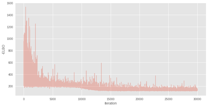
Results can be easily reused for another task, for example, using them to make predictions:
# x = tt.matrix('X') # n = tt.iscalar('n') # compute_test_value='raise', , x.tag.test_value = np.empty_like(X_train[:10]) n.tag.test_value = 100 # sample_node apply_replacements # pymc3 _sample_proba = approx.sample_node(get_output(p).flatten(), size=n, more_replacements={input_var:x}) # # , sample_proba = theano.function([x, n], _sample_proba) Actually the predictions themselves can be obtained by calling a function on the test set:
pred = sample_proba(X_test, 500).mean(0) > 0.5 fig, ax = plt.subplots() ax.scatter(X_test[pred==0, 0], X_test[pred==0, 1], color='b') ax.scatter(X_test[pred==1, 0], X_test[pred==1, 1], color='r') sns.despine() ax.set(title='Predicted labels in testing set', xlabel='X', ylabel='Y'); 
Dividing line
You can see the dividing border for classes, for this you can substitute there all the points on the plane and average.
grid = np.mgrid[-3:3:100j,-3:3:100j].astype('float32') grid_2d = grid.reshape(2, -1).T ppc = sample_proba(grid_2d ,500) cmap = sns.diverging_palette(250, 12, s=85, l=25, as_cmap=True) fig, ax = plt.subplots(figsize=(16, 9)) contour = ax.contourf(grid[0], grid[1], ppc.mean(axis=0).reshape(100, 100), cmap=cmap) ax.scatter(X_test[pred==0, 0], X_test[pred==0, 1], color='b') ax.scatter(X_test[pred==1, 0], X_test[pred==1, 1], color='r') cbar = plt.colorbar(contour, ax=ax) _ = ax.set(xlim=(-3, 3), ylim=(-3, 3), xlabel='X', ylabel='Y'); cbar.ax.set_ylabel('Posterior predictive mean probability of class label = 0'); 
Model confidence
Model confidence in predictions is a very interesting thing. Usually in models we can get only a point estimate for the value of interest. It does not in itself carry information about how well the model understands the world around it: only the distribution of the estimate can tell about it. Using Bayesian methods, this is done very intuitively, and, moreover, is pretty well implemented in PyMC3 .
cmap = sns.cubehelix_palette(light=1, as_cmap=True) fig, ax = plt.subplots(figsize=(16, 9)) contour = ax.contourf(grid[0], grid[1], ppc.std(axis=0).reshape(100, 100), cmap=cmap) ax.scatter(X_test[pred==0, 0], X_test[pred==0, 1], color='b') ax.scatter(X_test[pred==1, 0], X_test[pred==1, 1], color='r') cbar = plt.colorbar(contour, ax=ax) _ = ax.set(xlim=(-3, 3), ylim=(-3, 3), xlabel='X', ylabel='Y'); cbar.ax.set_ylabel('Uncertainty (posterior predictive standard deviation)'); 
, PyMC3. , , LDA .
- Bayesian Methods for Hackers
- Weight Uncertainty in Neural Networks
- Automatic Differentiation Variational Inference
- Operator Variational Inference
- Stein Variational Gradient Descent
- jupyter
Thanks
')
Source: https://habr.com/ru/post/322716/
All Articles