Open machine learning course. Topic 3. Classification, decision trees and the method of nearest neighbors
Hello to everyone who takes a course of machine learning in Habré!
In the first two parts ( 1 , 2 ) we practiced in the primary analysis of data with Pandas and in the construction of pictures, allowing to draw conclusions from the data. Today we finally move on to machine learning. Let's talk about machine learning tasks and consider 2 simple approaches - decision trees and the method of nearest neighbors. We also discuss how to choose a model for specific data using cross-validation.
UPD: now the course is in English under the brand mlcourse.ai with articles on Medium, and materials on Kaggle ( Dataset ) and on GitHub .
Video recording of the lecture based on this article in the second run of the open course (September-November 2017).
- Primary data analysis with Pandas
- Visual data analysis with Python
- Classification, decision trees and the method of nearest neighbors
- Linear classification and regression models
- Compositions: bagging, random forest
- Construction and selection of signs
- Teaching without a teacher: PCA, clustering
- Training in gigabytes with Vowpal Wabbit
- Time Series Analysis with Python
- Gradient boosting
Plan for this article:
- Introduction
- Decision tree
- Nearest Neighbor Method
- Selection of model parameters and cross-validation
- Application examples
- Pros and cons of decision trees and the method of nearest neighbors
- Homework number 3
- Useful resources
Introduction
Probably, I want to immediately rush into battle, but first we will talk about exactly what task we will solve and what is its place in the field of machine learning.
The classic, general (and not painfully strict) definition of machine learning sounds like (T. Mitchell "Machine learning", 1997):
they say that a computer program is trained in solving some problem from class T , if its performance, according to metric P , improves with accumulation of experience E.
Further, in different scenarios, T, P , and E imply completely different things. Among the most popular tasks of T in machine learning :
- classification - assignment of an object to one of the categories based on its characteristics
- regression - forecasting the quantitative characteristic of an object based on its other characteristics
- clustering - splitting a set of objects into groups based on the characteristics of these objects so that within groups the objects are similar to each other, and outside of one group they are less similar
- detection of anomalies - search for objects "strongly unlike" all others in the sample or some group of objects
- and many others more specific. A good overview is given in the chapter "Machine Learning basics" of the book "Deep Learning" (Ian Goodfellow, Yoshua Bengio, Aaron Courville, 2016)
Experience E means data (without them nowhere), and depending on this, machine learning algorithms can be divided into those that are trained with a teacher and without a teacher (supervised and unsupervised learning). In the tasks of learning without a teacher, there is a sample consisting of objects described by a set of features . In addition to this, for each object of a certain sample, called a training one , the target attribute is known in the tasks of training with a teacher - in fact, this is what I would like to predict for other objects that are not from a training sample.
Example
The tasks of classification and regression are the problems of learning with a teacher. As an example, we will present the task of credit scoring: on the basis of data accumulated by a credit institution about its customers, we would like to predict loan default. Here, for the algorithm, experience E is the available training sample: a set of objects (people), each of which is characterized by a set of attributes (such as age, salary, type of credit, defaults in the past, etc.), as well as a target attribute . If this target sign is simply a fact of non-repayment of a loan (1 or 0, that is, the bank knows about its customers, who repaid the loan and who does not), then this is the (binary) classification task. If it is known how long the client has delayed the return of the loan and would like to predict the same for new clients, then this will be a regression task.
Finally, the third abstraction in the definition of machine learning is the metrics for evaluating the performance of the algorithm P. Such metrics differ for different tasks and algorithms, and we will talk about them as we study the algorithms. So far we say that the simplest metric of the quality of the algorithm that solves the classification problem is the proportion of correct answers ( accuracy , do not call it accuracy , this translation is reserved for another metric, precision ) - that is, simply the proportion of correct predictions of the algorithm on the test sample.
Further we will talk about two tasks of teaching with a teacher: about classification and regression.
Decision tree
Let us begin the review of the methods of classification and regression with one of the most popular - the decision tree. Decision trees are used in everyday life in the most diverse areas of human activity, sometimes very far from machine learning. Decision tree can be called visual instruction what to do in what situation. Let us give an example from the field of consulting research institutes. The Higher School of Economics publishes info-schemes that make life easier for its employees. Here is a fragment of the instruction for publishing a scientific article on the institute portal.

In terms of machine learning, we can say that this is an elementary classifier that determines the form of publication on the portal (book, article, chapter of the book, preprint, publication in the HSE and the Media) on several grounds: type of publication (monograph, brochure, article and etc.), the type of publication in which the article was published (a scientific journal, a collection of papers, etc.) and the rest.
Often, a decision tree serves as a synthesis of expert experience, a means of transferring knowledge to future employees or a model of a company's business process. For example, prior to the introduction of scalable machine learning algorithms in the banking sector, the task of credit scoring was solved by experts. The decision to issue a loan to the borrower was made on the basis of some intuitively (or by experience) derived rules that can be represented as a decision tree.
In this case, we can say that the binary classification problem is being solved (the target class has two meanings: “Issue a loan” and “Refuse”) according to the signs “Age”, “Home”, “Income” and “Education”.
A decision tree as an algorithm for machine learning is essentially the same: a combination of logical rules of the form "Meaning of a feature a less x And Sign Value b less y ... => Class 1 "in the data structure" Tree ". The tremendous advantage of decision trees is that they are easily interpretable, understandable to man. For example, according to the diagram in the figure above, you can explain to the borrower why he was denied a loan. For example, that he does not have a home and an income of less than 5,000. As we will see later, many other, albeit more accurate, models do not have this property and can rather be viewed as a “black box” into which they downloaded data and received an answer. "clear" decision trees and their similarity to the model adopted solutions by man (you can easily explain your model to the boss), decision trees have gained immense popularity, and one of the representatives of this group of classification methods, C4.5, is considered first in the list of the top 10 data mining algorithms ("Top 10 algorithms in data mining", Knowledge and Information Systems, 2008. PDF ).
How the decision tree is built
In the example of credit scoring, we saw that the decision to issue a loan was made on the basis of age, availability of real estate, income, and others. But which sign to choose first? To do this, consider an example more simply, where all the signs are binary.
Here you can recall the game "20 questions", which is often mentioned in the introduction to decision trees. Surely everyone was playing it. One person makes a celebrity, and the second one tries to guess by asking only questions that can be answered with “Yes” or “No” (omitting the options “I don’t know” and “I can’t say”). What question guesses ask the first thing? Of course, one that will reduce the number of remaining options the most. For example, the question "Is this Angelina Jolie?" in the case of a negative answer, it will leave more than 7 billion options for further search (of course, smaller, not every person is a celebrity, but still a lot), but the question "Is this a woman?" already cut off about half of the celebrities. That is, the sign "gender" is much better shared by a sample of people than the sign "this is Angelina Jolie", "Spanish nationality" or "likes football". This is intuitively consistent with the concept of information gain based on entropy.
Entropy
Shannon entropy is determined for a system with N possible states as follows:
LargeS=− sumNi=1pi log2pi,
Where pi - probability of finding the system in i -th state. This is a very important concept used in physics, information theory and other fields. Omitting the premises of the introduction (combinatorial and information-theoretic) of this concept, we note that, intuitively, entropy corresponds to the degree of chaos in the system. The higher the entropy, the less ordered the system and vice versa. This will help us to formalize the "effective sampling division," which we talked about in the context of the 20 questions game.
Example
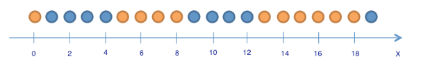
To illustrate how entropy will help identify good signs for building a tree, we’ll give the same toy example as in the article "Entropy and Decision Trees" . We will predict the color of the ball according to its coordinate. Of course, it has nothing to do with life, but it does allow showing how entropy is used to build a decision tree.
')
There are 9 blue balls and 11 yellow balls. If we pulled a ball at random, then with probability p1= frac920 will be blue and with probability p2= frac1120 - yellow. So the state entropy S0=− frac920 log2 frac920− frac1120 log2 frac1120 approx1 . This value itself does not tell us anything yet. Now let's see how the entropy changes, if the balls are divided into two groups - with a coordinate less than or equal to 12 and more than 12.
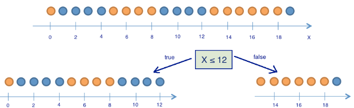
In the left group were 13 balls, of which 8 are blue and 5 are yellow. The entropy of this group is equal to S1=− frac513 log2 frac513− frac813 log2 frac813 approx$0.9 . In the right group were 7 balls, of which 1 is blue and 6 are yellow. The entropy of the right group is S2=− frac17 log2 frac17− frac67 log2 frac67 approx0.6 . As you can see, the entropy decreased in both groups as compared with the initial state, although not much in the left state. Since entropy is essentially a degree of chaos (or uncertainty) in a system, a decrease in entropy is called an increase in information. Formally, the increase in information (information gain, IG) when dividing the sample on the basis of Q (in our example, this is a sign " x leq12 ") is defined as
LargeIG(Q)=SO− sumqi=1 fracNiNSi,
Where q - the number of groups after splitting, Ni - the number of sample elements in which the sign Q It has i th value. In our case, after the separation, we got two groups ( q=2 ) - one of 13 elements ( N1=13 ), the second - from 7 ( N2=7 ). The increase in information turned out
LargeIG(x leq12)=S0− frac1320S1− frac720S2 approx0.16.
It turns out that by dividing the balls into two groups on the basis of "the coordinate is less or equal to 12", we have already received a more ordered system than at the beginning. We continue the division of the balls into groups until the balls in each group are of the same color.

For the right group, it took only one additional splitting on the basis of "the coordinate is less or equal to 18", for the left group - three more. Obviously, the entropy of a group with balls of the same color is 0 ( log21=0 ), which corresponds to the notion that a group of balls of the same color is ordered.
As a result, we built a decision tree that predicts the color of the ball according to its coordinate. Note that such a decision tree can work poorly for new objects (determining the color of new balls), since it ideally adjusted to the training sample (the original 20 balls). To classify new balls, a tree with a smaller number of “questions” or divisions will be better suited, even if it does not ideally divide the training set by color. This problem, retraining, we will look further.
Tree building algorithm
One can be convinced that the tree constructed in the previous example is in a certain sense optimal - only 5 "questions" were required (conditions for the sign x ) to "fit" the decision tree under the training sample, that is, so that the tree correctly classifies any training object. Under other conditions of sampling separation, the tree will turn out deeper.
The basis of popular decision-making algorithms, such as ID3 and C4.5, is the principle of greedily maximizing the growth of information - at each step, the feature is chosen, when divided into which information growth is greatest. Then the procedure is repeated recursively until the entropy is zero or some small value (unless the tree is ideally fitted to the training set in order to avoid retraining).
Different algorithms use different heuristics for "early stopping" or "clipping" to avoid building a retrained tree.
def build(L): create node t if the stopping criterion is True: assign a predictive model to t else: Find the best binary split L = L_left + L_right t.left = build(L_left) t.right = build(L_right) return t Other breakdown quality criteria in the classification task
We understand how the concept of entropy allows us to formalize the idea of the quality of a partition in a tree. But this is just a heuristic, there are others:
- Gini impurity: G=1− sum limitsk(pk)2 . The maximization of this criterion can be interpreted as maximizing the number of pairs of objects of the same class that are in the same subtree. You can learn more about this (as well as about many other things) from the repository of Evgeny Sokolov. Not to be confused with the Gini index! Read more about this confusion - the blog post Alexander Dyakonov
- Misclassification error: E=1− max limitskpk
In practice, the classification error is almost not used, and the Gini uncertainty and the increase in information work almost equally.
In the case of a binary classification problem ( p+ - the probability of an object to have a label +) entropy and Gini uncertainty will take the following form:
S=−p+ log2p+−p− log2p−=−p+ log2p+−(1−p+) log2(1−p+);
G=1−p2+−p2−=1−p2+−(1−p+)2=2p+(1−p+).
When we build graphs of two functions of the argument p+ then we will see that the entropy graph is very close to the Gini double uncertainty graph, and therefore in practice these two criteria “work” almost equally.
from __future__ import division, print_function # Anaconda import warnings warnings.filterwarnings('ignore') import numpy as np import pandas as pd %matplotlib inline import seaborn as sns from matplotlib import pyplot as plt plt.rcParams['figure.figsize'] = (6,4) xx = np.linspace(0,1,50) plt.plot(xx, [2 * x * (1-x) for x in xx], label='gini') plt.plot(xx, [4 * x * (1-x) for x in xx], label='2*gini') plt.plot(xx, [-x * np.log2(x) - (1-x) * np.log2(1 - x) for x in xx], label='entropy') plt.plot(xx, [1 - max(x, 1-x) for x in xx], label='missclass') plt.plot(xx, [2 - 2 * max(x, 1-x) for x in xx], label='2*missclass') plt.xlabel('p+') plt.ylabel('criterion') plt.title(' p+ ( )') plt.legend(); 
Example
Consider an example of using the decision tree from the Scikit-learn library for synthetic data. Two classes will be generated from two normal distributions with different means.
# np.seed = 7 train_data = np.random.normal(size=(100, 2)) train_labels = np.zeros(100) # train_data = np.r_[train_data, np.random.normal(size=(100, 2), loc=2)] train_labels = np.r_[train_labels, np.ones(100)] Display the data. Informally, the task of classification in this case is to build some kind of "good" border separating 2 classes (red points from yellow ones). If to exaggerate, machine learning in this case comes down to how to choose a good dividing border. Perhaps the straight line will be too simple a boundary, and some complex curve that goes around every red dot will be too complicated and we will make a lot of mistakes on new examples from the same distribution from which the training sample came. Intuition tells you that some kind of smooth border separating 2 classes, or at least just a straight line (in n -dimensional case - hyperplane).
plt.rcParams['figure.figsize'] = (10,8) plt.scatter(train_data[:, 0], train_data[:, 1], c=train_labels, s=100, cmap='autumn', edgecolors='black', linewidth=1.5); plt.plot(range(-2,5), range(4,-3,-1)); 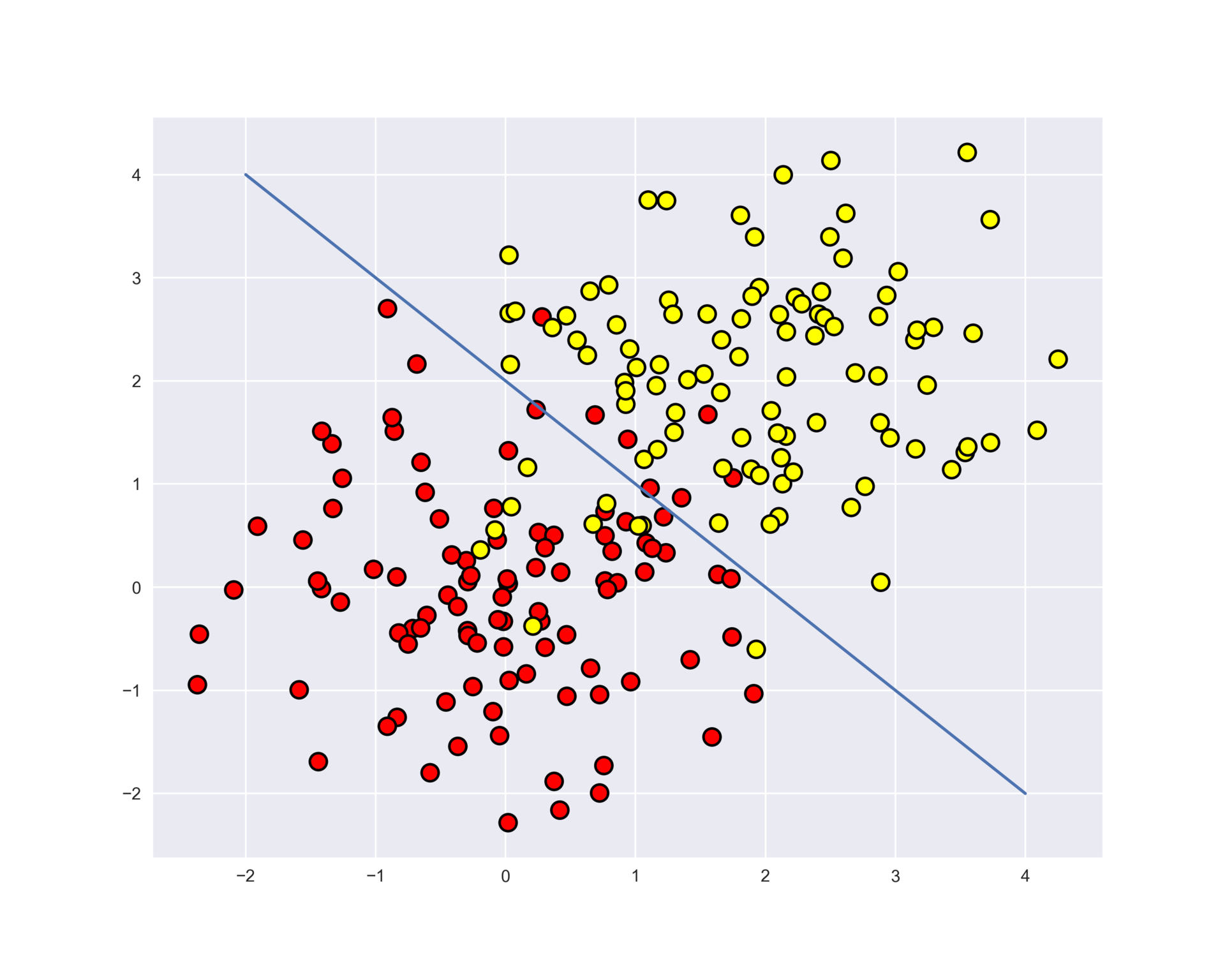
Let's try to separate these two classes, having trained a decision tree. In the tree, we will use the max_depth parameter, which limits the depth of the tree. Visualize the resulting class separation boundary.
from sklearn.tree import DecisionTreeClassifier # , . def get_grid(data): x_min, x_max = data[:, 0].min() - 1, data[:, 0].max() + 1 y_min, y_max = data[:, 1].min() - 1, data[:, 1].max() + 1 return np.meshgrid(np.arange(x_min, x_max, 0.01), np.arange(y_min, y_max, 0.01)) # min_samples_leaf , # clf_tree = DecisionTreeClassifier(criterion='entropy', max_depth=3, random_state=17) # clf_tree.fit(train_data, train_labels) # xx, yy = get_grid(train_data) predicted = clf_tree.predict(np.c_[xx.ravel(), yy.ravel()]).reshape(xx.shape) plt.pcolormesh(xx, yy, predicted, cmap='autumn') plt.scatter(train_data[:, 0], train_data[:, 1], c=train_labels, s=100, cmap='autumn', edgecolors='black', linewidth=1.5); 
And what does a self-made tree look like? We see that the tree "cuts" the space into 7 rectangles (there are 7 leaves in the tree). In each such rectangle, the tree forecast will be constant, according to the prevalence of objects of a particular class.
# .dot from sklearn.tree import export_graphviz export_graphviz(clf_tree, feature_names=['x1', 'x2'], out_file='../../img/small_tree.dot', filled=True) # pydot (pip install pydot) !dot -Tpng '../../img/small_tree.dot' -o '../../img/small_tree.png' 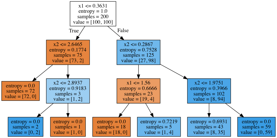
How does a tree “read”?
In the beginning there were 200 objects, 100 - of one class and 100 - of another. The entropy of the initial state was maximum - 1. Then, the objects were divided into 2 groups depending on the comparison of the sign x1 with value 0.3631 (find this section of the border in the figure above, before the tree). At the same time, the entropy in the left and in the right group of objects decreased. And so on, the tree is built to a depth of 3. With such visualization, the more objects of one class, the vertex color is closer to dark orange and, conversely, the more objects of the second class, the closer the color to dark blue. At the beginning of the objects of one class equally, therefore the root of the tree is white.
How a decision tree works with quantitative attributes
Suppose there is a quantitative attribute "Age" in the sample, which has many unique values. The decision tree will look for the best (according to the criterion of the type of information growth) sampling, checking binary signs such as "Age <17", "Age <22.87", etc. But what if there are too many of these "cuts" of age? And what if there is still a quantitative sign "Salary", and the salary can also be "cut" in a large number of ways? It turns out too many binary features to select the best at each step of building a tree. To solve this problem, heuristics are used to limit the number of thresholds with which we compare a quantitative trait.
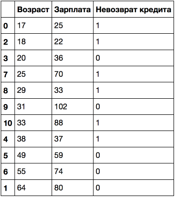
Consider this on a toy example. Let there be the following sample:
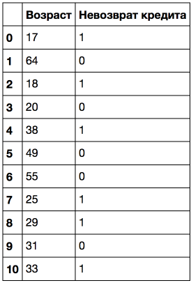
Sort it by increasing age.

Let's teach a decision tree on this data (without limiting the depth) and look at it.
age_tree = DecisionTreeClassifier(random_state=17) age_tree.fit(data[''].values.reshape(-1, 1), data[' '].values) export_graphviz(age_tree, feature_names=[''], out_file='../../img/age_tree.dot', filled=True) !dot -Tpng '../../img/age_tree.dot' -o '../../img/age_tree.png' In the picture below we see that the tree used 5 values with which the age is compared: 43.5, 19, 22.5, 30 and 32 years. If you look closely, then this is exactly the average values between the ages at which the target class "changes" from 1 to 0 or vice versa. Difficult phrase, so an example: 43.5 is the average between 38 and 49 years old, the client who was not returned a loan for 38 years, and the one to whom 49 returned. Likewise, 19 years is an average between 18 and 20 years. That is, as thresholds for “cutting” a quantitative trait, the tree “looks” at those values at which the target class changes its value.
Think about why it does not make sense in this case to consider the sign "Age <17.5".

Consider an example more complicated: add the sign "Salary" (thousand rubles / month).
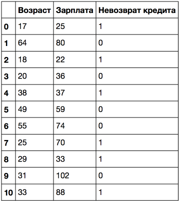
If you sort by age, the target class ("Loan non-repayment") changes (from 1 to 0 or vice versa) 5 times. And if you sort by salary - then 7 times. How will the tree now select signs? We'll see.

age_sal_tree = DecisionTreeClassifier(random_state=17) age_sal_tree.fit(data2[['', '']].values, data2[' '].values); export_graphviz(age_sal_tree, feature_names=['', ''], out_file='../../img/age_sal_tree.dot', filled=True) !dot -Tpng '../../img/age_sal_tree.dot' -o '../../img/age_sal_tree.png' 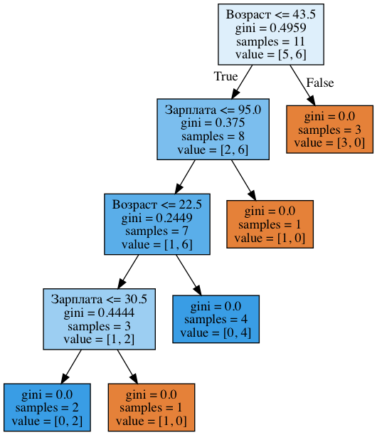
We see that the tree involved as a breakdown of age and salary. And the thresholds with which the signs are compared: 43.5 and 22.5 years - for the age and 95 and 30.5 thousand rubles / month - for the salary. And again it can be noted that 95 thousand is the average between 88 and 102, while the person with a salary of 88 turned out to be “bad”, and from 102 - “good”. The same is true for 30.5 thousand. That is, the comparison of wages and age did not go with all possible values, but only with a few. Why did these signs appear in the tree? Because the breaks for them turned out to be better (according to the Gini criterion of uncertainty).
Conclusion: the simplest heuristics for processing quantitative attributes in the decision tree: the quantitative attribute is sorted in ascending order, and only those thresholds are checked in the tree at which the target characteristic changes value. It does not sound very strict, but I hope I brought the meaning with the help of toy examples.
In addition, when there are many quantitative features in the data, and each has many unique values, not all the thresholds described above can be selected, but only the top-N, which give the maximum gain of the same criterion. That is, in fact, for each threshold, a tree of depth 1 is built, it is considered how much the entropy (or Gini uncertainty) has decreased and only the best thresholds are selected with which to compare the quantitative trait.
For illustration: when splitting on the basis of "Salary leq 34.5 "entropy 0 in the left subgroup (all clients are" bad "), and in the right subgroup - 0.954 (3" bad "and 5" good ", you can check, 1 part of the homework will be just to sort out the construction of trees ). The increase in information is obtained approximately 0.3.
And when splitting on the basis of "Salary leq 95 "in the left subgroup is entropy 0.97 (6" bad "and 4" good "), and in the right - 0 (only one object). The increase in information is approximately 0.11.
Considering the increase in information for each partition in this way, it is possible to select, before building a large tree (for all attributes), thresholds with which each quantitative attribute will be compared.
More examples of quantifying quantitative traits can be viewed in posts similar to this or that . One of the most famous scientific articles on this topic is "On the handling of continuous-valued attributes in decision tree generation" (UM Fayyad. KB Irani, "Machine Learning", 1992).
The main parameters of the tree
In principle, a decision tree can be built to such a depth that there is exactly one object in each sheet. But in practice this is not done (if only one tree is built) due to the fact that such a tree will be retrained - it will be too tuned in to the training set and will not work well on the forecast on new data. Somewhere at the bottom of the tree, at a great depth, breaks will appear on less important grounds (for example, whether a client came from Saratov or Kostroma). If you exaggerate, it may turn out that of all 4 clients who came to the bank for a loan in green pants, no one returned the loan. But we do not want our classification model to generate such specific rules.
There are two exceptions, situations where trees are built to maximum depth:
- Random forest (the composition of many trees) averages the answers of trees built to the maximum depth (why you should do this, we will understand later)
- Tree trimming ( pruning ). With this approach, the tree is first built to the maximum depth, then gradually, from bottom to top, some tree tops are removed by comparing the quality of the tree with this partition and without it (the comparison is carried out using cross-validation , about which just below). You can read more in the materials of the repository of Evgeny Sokolov.
The image below is an example of a dividing boundary built by a retrained tree.

The main ways to combat retraining in the case of decision trees are:
- artificial limitation of the depth or the minimum number of objects in the sheet: the tree is simply stopped at some point;
- tree trimming
DecisionTreeClassifier class in Scikit-learn
The main parameters of the class sklearn.tree.DecisionTreeClassifier :
max_depth- maximum tree depthmax_features- the maximum number of features by which the best partitioning in the tree is sought (this is necessary because with a large number of attributes it will be “expensive” to search for the best (by the criterion of the type of information growth) the partitioning among all features)min_samples_leaf- the minimum number of objects in the sheet. This parameter has a clear interpretation: for example, if it is 5, then the tree will generate only those classifying rules that are valid for at least 5 objects
Tree parameters must be adjusted depending on the input data, and this is usually done using cross-validation , about it just below.
Decision tree in the regression problem
When predicting a quantitative trait, the idea of building a tree remains the same, but the quality criterion changes:
- Dispersion around the middle: LargeD= frac1 ell sum limits elli=1(yi− frac1 ell sum limits elli=1yi)2,
Where ell - the number of objects in the sheet, yi - values of the target feature. Simply put, by minimizing the variance around the mean, we look for signs that break the sample in such a way that the values of the target characteristic in each sheet are approximately equal.
Example
Generate data distributed around the function. f(x)=e−x2+1.5∗e−(x−2)2 with some noise, we will teach them a decision tree and we will depict what forecasts the tree makes.
n_train = 150 n_test = 1000 noise = 0.1 def f(x): x = x.ravel() return np.exp(-x ** 2) + 1.5 * np.exp(-(x - 2) ** 2) def generate(n_samples, noise): X = np.random.rand(n_samples) * 10 - 5 X = np.sort(X).ravel() y = np.exp(-X ** 2) + 1.5 * np.exp(-(X - 2) ** 2) + \ np.random.normal(0.0, noise, n_samples) X = X.reshape((n_samples, 1)) return X, y X_train, y_train = generate(n_samples=n_train, noise=noise) X_test, y_test = generate(n_samples=n_test, noise=noise) from sklearn.tree import DecisionTreeRegressor reg_tree = DecisionTreeRegressor(max_depth=5, random_state=17) reg_tree.fit(X_train, y_train) reg_tree_pred = reg_tree.predict(X_test) plt.figure(figsize=(10, 6)) plt.plot(X_test, f(X_test), "b") plt.scatter(X_train, y_train, c="b", s=20) plt.plot(X_test, reg_tree_pred, "g", lw=2) plt.xlim([-5, 5]) plt.title("Decision tree regressor, MSE = %.2f" % np.sum((y_test - reg_tree_pred) ** 2)) plt.show() 
We see that the decision tree approximates the dependence in the data by a piecewise constant function.
Nearest Neighbor Method
The Neighbor Neighbor Method (kNN) is also a very popular classification method, also sometimes used in regression tasks. This, along with the decision tree, is one of the most understandable approaches to classification. At the level of intuition, the essence of the method is as follows: look at the neighbors that prevail, and so do you. Formally, the basis of the method is the compactness hypothesis: if the metric of the distance between the examples is introduced quite successfully, then similar examples are more often in the same class than in the other.
According to the method of the nearest neighbors, the test example (green ball) will be classified as “blue”, not “red”.

For example, if you don’t know what type of product to specify in the ad for a Bluetooth headset, you can find 5 similar headsets, and if 4 of them are categorized as “Accessories”, and only one - into the category “Technique”, common sense will tell your ad also indicate the category "Accessories".
To classify each of the test sample objects, you must perform the following operations sequentially:
- Calculate the distance to each of the objects of the training sample
- Take away k objects of the training sample, the distance to which the minimum
- The class of the object being classified is the class most often found among k closest neighbors
The method adapts to the regression task quite easily - at step 3, it is not the label that returns, but the number - the average (or median) value of the target attribute among the neighbors.
A notable feature of this approach is its laziness. This means that the calculations begin only at the moment of the classification of the test case, and in advance, only if there are training examples, no model is built. This is different, for example, from the previously considered decision tree, where first a tree is built on the basis of a training sample, and then the test case is classified relatively quickly.
It is worth noting that the method of nearest neighbors is a well-studied approach (in machine learning, econometrics and statistics, more is known, probably, only about linear regression). For the method of nearest neighbors, there are quite a few important theorems that state that on "infinite" samples this is the optimal classification method. The authors of the classic book "The Elements of Statistical Learning" consider kNN to be a theoretically ideal algorithm, the applicability of which is simply limited by computational capabilities and the curse of dimensions.
The method of nearest neighbors in real problems
- In its pure form, kNN can serve as a good start (baseline) in solving a problem;
- In Kaggle competitions, kNN is often used to build meta-attributes (the kNN prediction is input to other models) or in stacking / blending;
- The idea of the nearest neighbor extends to other tasks, for example, in recommender systems, a simple initial solution may be to recommend some product (or service) popular among the nearest neighbors of the person to whom we want to make a recommendation;
- In practice, for large samples often use approximate methods of finding the nearest neighbors. Here is a lecture by Artyom Babenko about efficient algorithms for finding the nearest neighbors among billions of objects in high-dimensional spaces (search by pictures). Also known are open libraries in which these algorithms are implemented, thanks to Spotify for its Annoy library.
/ :
- ( , , ). , . , "" 100 , "" 100.
- ( , , , "")
KNeighborsClassifier Scikit-learn
sklearn.neighbors.KNeighborsClassifier:
- weights: "uniform" ( ), "distance" ( )
- algorithm (): "brute", "ball_tree", "KD_tree", "auto". . — , . "auto" .
- leaf_size (): BallTree KDTree
- metric: "minkowski", "manhattan", "euclidean", "chebyshev"
-
– , . ( , ), , .
2 :
- ( held-out/hold-out set ). - ( 20% 40%), (60-80% ) (, – ) .
- - ( cross-validation , ). – K-fold -

K ( K−1 ) ( ), ( , ).
K , , / -.
- . - , .
- – ( ), , , .. , , Sebastian Raschka ()
-
DataFrame . Series, . , , .
df = pd.read_csv('../../data/telecom_churn.csv') df['International plan'] = pd.factorize(df['International plan'])[0] df['Voice mail plan'] = pd.factorize(df['Voice mail plan'])[0] df['Churn'] = df['Churn'].astype('int') states = df['State'] y = df['Churn'] df.drop(['State', 'Churn'], axis=1, inplace=True) 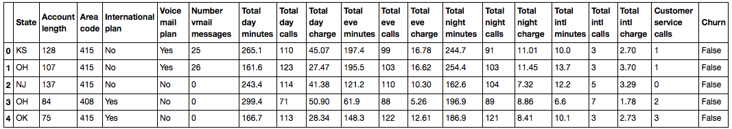
70% (X_train, y_train) 30% (X_holdout, y_holdout). , , , . 2 – kNN, , , : 5, – 10.
from sklearn.model_selection import train_test_split, StratifiedKFold from sklearn.neighbors import KNeighborsClassifier X_train, X_holdout, y_train, y_holdout = train_test_split(df.values, y, test_size=0.3, random_state=17) tree = DecisionTreeClassifier(max_depth=5, random_state=17) knn = KNeighborsClassifier(n_neighbors=10) tree.fit(X_train, y_train) knn.fit(X_train, y_train) – . . : 94% 88% kNN. .
from sklearn.metrics import accuracy_score tree_pred = tree.predict(X_holdout) accuracy_score(y_holdout, tree_pred) # 0.94 knn_pred = knn.predict(X_holdout) accuracy_score(y_holdout, knn_pred) # 0.88 -. . , GridSearchCV: max_depth max_features 5- - .
from sklearn.model_selection import GridSearchCV, cross_val_score tree_params = {'max_depth': range(1,11), 'max_features': range(4,19)} tree_grid = GridSearchCV(tree, tree_params, cv=5, n_jobs=-1, verbose=True) tree_grid.fit(X_train, y_train) -:
tree_grid.best_params_ {'max_depth': 6, 'max_features': 17}
tree_grid.best_score_ 0.94256322331761677
accuracy_score(y_holdout, tree_grid.predict(X_holdout)) 0.94599999999999995
kNN.
from sklearn.pipeline import Pipeline from sklearn.preprocessing import StandardScaler knn_pipe = Pipeline([('scaler', StandardScaler()), ('knn', KNeighborsClassifier(n_jobs=-1))]) knn_params = {'knn__n_neighbors': range(1, 10)} knn_grid = GridSearchCV(knn_pipe, knn_params, cv=5, n_jobs=-1, verbose=True) knn_grid.fit(X_train, y_train) knn_grid.best_params_, knn_grid.best_score_ ({'knn__n_neighbors': 7}, 0.88598371195885128)
accuracy_score(y_holdout, knn_grid.predict(X_holdout)) 0.89000000000000001
, : 94.2% - 94.6% 88.6% / 89% kNN. , , ( , - , ) (95.1% - 95.3% – ), .
from sklearn.ensemble import RandomForestClassifier forest = RandomForestClassifier(n_estimators=100, n_jobs=-1, random_state=17) print(np.mean(cross_val_score(forest, X_train, y_train, cv=5))) # 0.949 forest_params = {'max_depth': range(1,11), 'max_features': range(4,19)} forest_grid = GridSearchCV(forest, forest_params, cv=5, n_jobs=-1, verbose=True) forest_grid.fit(X_train, y_train) forest_grid.best_params_, forest_grid.best_score_ # ({'max_depth': 9, 'max_features': 6}, 0.951) accuracy_score(y_holdout, forest_grid.predict(X_holdout)) # 0.953 . - , ( – 6), , "", .
export_graphviz(tree_grid.best_estimator_, feature_names=df.columns, out_file='../../img/churn_tree.dot', filled=True) !dot -Tpng '../../img/churn_tree.dot' -o '../../img/churn_tree.png' 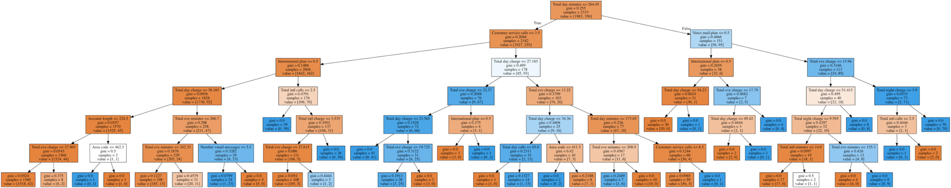
, , - "", . (2 ), (+1, , -1 – ). , – .
def form_linearly_separable_data(n=500, x1_min=0, x1_max=30, x2_min=0, x2_max=30): data, target = [], [] for i in range(n): x1, x2 = np.random.randint(x1_min, x1_max), np.random.randint(x2_min, x2_max) if np.abs(x1 - x2) > 0.5: data.append([x1, x2]) target.append(np.sign(x1 - x2)) return np.array(data), np.array(target) X, y = form_linearly_separable_data() plt.scatter(X[:, 0], X[:, 1], c=y, cmap='autumn', edgecolors='black'); 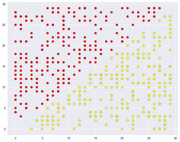
. , , 30×30 , .
tree = DecisionTreeClassifier(random_state=17).fit(X, y) xx, yy = get_grid(X, eps=.05) predicted = tree.predict(np.c_[xx.ravel(), yy.ravel()]).reshape(xx.shape) plt.pcolormesh(xx, yy, predicted, cmap='autumn') plt.scatter(X[:, 0], X[:, 1], c=y, s=100, cmap='autumn', edgecolors='black', linewidth=1.5) plt.title('Easy task. Decision tree compexifies everything'); 
, ( ) – x1=x2 .
export_graphviz(tree, feature_names=['x1', 'x2'], out_file='../../img/deep_toy_tree.dot', filled=True) !dot -Tpng '../../img/deep_toy_tree.dot' -o '../../img/deep_toy_tree.png' 
, , ( ).
knn = KNeighborsClassifier(n_neighbors=1).fit(X, y) xx, yy = get_grid(X, eps=.05) predicted = knn.predict(np.c_[xx.ravel(), yy.ravel()]).reshape(xx.shape) plt.pcolormesh(xx, yy, predicted, cmap='autumn') plt.scatter(X[:, 0], X[:, 1], c=y, s=100, cmap='autumn', edgecolors='black', linewidth=1.5); plt.title('Easy task, kNN. Not bad'); 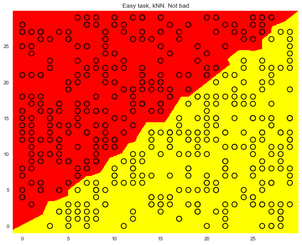
MNIST
2 . "" sklearn . , .
8 x 8 ( ). "" 64, .
, , .
from sklearn.datasets import load_digits data = load_digits() X, y = data.data, data.target X[0,:].reshape([8,8]) array([[ 0., 0., 5., 13., 9., 1., 0., 0.],
[ 0., 0., 13., 15., 10., 15., 5., 0.],
[ 0., 3., 15., 2., 0., 11., 8., 0.],
[ 0., 4., 12., 0., 0., 8., 8., 0.],
[ 0., 5., 8., 0., 0., 9., 8., 0.],
[ 0., 4., 11., 0., 1., 12., 7., 0.],
[ 0., 2., 14., 5., 10., 12., 0., 0.],
[ 0., 0., 6., 13., 10., 0., 0., 0.]])
f, axes = plt.subplots(1, 4, sharey=True, figsize=(16,6)) for i in range(4): axes[i].imshow(X[i,:].reshape([8,8])); 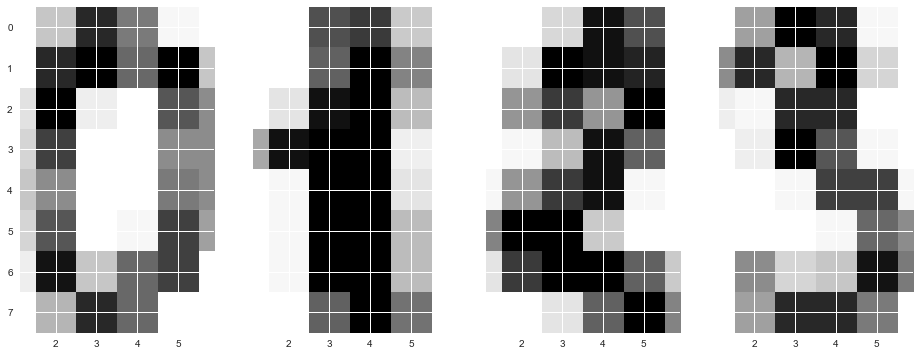
, , .
70% (X_train, y_train) 30% (X_holdout, y_holdout). , , , .
X_train, X_holdout, y_train, y_holdout = train_test_split(X, y, test_size=0.3, random_state=17) kNN, .
tree = DecisionTreeClassifier(max_depth=5, random_state=17) knn = KNeighborsClassifier(n_neighbors=10) tree.fit(X_train, y_train) knn.fit(X_train, y_train) . , . .
tree_pred = tree.predict(X_holdout) knn_pred = knn.predict(X_holdout) accuracy_score(y_holdout, knn_pred), accuracy_score(y_holdout, tree_pred) # (0.97, 0.666) , -, , , — 64.
tree_params = {'max_depth': [1, 2, 3, 5, 10, 20, 25, 30, 40, 50, 64], 'max_features': [1, 2, 3, 5, 10, 20 ,30, 50, 64]} tree_grid = GridSearchCV(tree, tree_params, cv=5, n_jobs=-1, verbose=True) tree_grid.fit(X_train, y_train) -:
tree_grid.best_params_, tree_grid.best_score_ # ({'max_depth': 20, 'max_features': 64}, 0.844) 66%, 97%. . - 99% .
np.mean(cross_val_score(KNeighborsClassifier(n_neighbors=1), X_train, y_train, cv=5)) # 0.987 , , . .
np.mean(cross_val_score(RandomForestClassifier(random_state=17), X_train, y_train, cv=5)) # 0.935 , , RandomForestClassifier, 98%, .
(: CV Holdout– - -. DT – , kNN – , RF – )
| CV | Holdout | |
|---|---|---|
| DT | 0.844 | 0.838 |
| kNN | 0.987 | 0.983 |
| RF | 0.935 | 0.941 |
( ): – ( ), , .
. , .
def form_noisy_data(n_obj=1000, n_feat=100, random_seed=17): np.seed = random_seed y = np.random.choice([-1, 1], size=n_obj) # x1 = 0.3 * y # – x_other = np.random.random(size=[n_obj, n_feat - 1]) return np.hstack([x1.reshape([n_obj, 1]), x_other]), y X, y = form_noisy_data() , - . , n_neighbors . .
, , . , "" .
from sklearn.model_selection import cross_val_score cv_scores, holdout_scores = [], [] n_neighb = [1, 2, 3, 5] + list(range(50, 550, 50)) for k in n_neighb: knn = KNeighborsClassifier(n_neighbors=k) cv_scores.append(np.mean(cross_val_score(knn, X_train, y_train, cv=5))) knn.fit(X_train, y_train) holdout_scores.append(accuracy_score(y_holdout, knn.predict(X_holdout))) plt.plot(n_neighb, cv_scores, label='CV') plt.plot(n_neighb, holdout_scores, label='holdout') plt.title('Easy task. kNN fails') plt.legend(); 
tree = DecisionTreeClassifier(random_state=17, max_depth=1) tree_cv_score = np.mean(cross_val_score(tree, X_train, y_train, cv=5)) tree.fit(X_train, y_train) tree_holdout_score = accuracy_score(y_holdout, tree.predict(X_holdout)) print('Decision tree. CV: {}, holdout: {}'.format(tree_cv_score, tree_holdout_score)) Decision tree. CV: 1.0, holdout: 1.0
, , . , , : , .
Pros:
- , , , " < 25 , ". ;
- , "" ( ) (), ( );
- ;
- ;
- , .
Minuses:
- : , , (, ), , ;
- , , ( , - ), ;
- (pruning) . , — ;
- . . ( );
- ( ) NP-, , ;
- . Friedman , 50% CART ( – Classification And Regression Trees,
sklearn); - , ( ). , , . , > 19 < 0.
Pros:
- ;
- ;
- , , , , , ;
- ( : , kNN ). , kNN, . ( , "VideoLectures.Net Recommender System Challenge") ;
- , , . : , (: " , 350 , 70 – , 12% , ").
Minuses:
- , , , , , , , (100-150), , ;
- , , /;
- . . , ;
- — (, ). , ;
- , , , - " ". ML- Pedro Domingos – "A Few Useful Things to Know about Machine Learning", "the curse of dimensionality" Deep Learning "Machine Learning basics".
, , . , .
№ 3
– , , , Adult UCI. - ( ).
Useful resources
- Open Machine Learning Course. Topic 3. Classification, Decision Trees and k Nearest Neighbors ( )
- – rushter . , , , ;
- ( GitHub). , ;
- GitHub (.). ;
- " " ;
- " . " .
Source: https://habr.com/ru/post/322534/
All Articles