Neural network imitation game
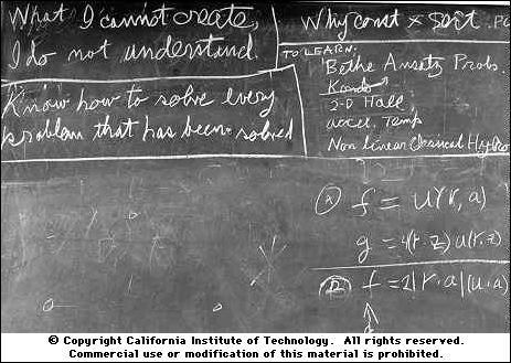 Hello colleagues. In the late 1960s, Richard Feynman gave a course of general physics in Caltech. Feynman agreed to read his course exactly once. The university understood that the lectures would be a historic event, undertook to write down all the lectures and photograph all the drawings that Feynman did on the blackboard. Maybe it was after this that the university had a habit of photographing all the boards that his hand touched. The photo on the right was taken in the year of Feynman's death. In the upper left corner it is written: " What I cannot create, I do not understand ". Not only physicists, but also biologists said this to themselves. In 2011, Craig Venter created the world's first synthetic living organism, i.e. The DNA of this organism is created by man. The body is not very big, just from one cell. In addition to all that is necessary for the reproduction of a vital activity program, the names of the creators, their emails, and Richard Feynman's quotation were coded into the DNA (albeit with an error, it was later corrected, by the way). Want to know what this cool is about here? I invite under kat, colleagues.
Introduction
Over the centuries, people have been trying to create things that cannot be explained in principle. The first real model of artificial intelligence, not at all mythical, and quite understandable as a worker, was Rosenblatt's perceptron . And then everything started spinning . Consider the field of computer vision in more detail. Today, neural networks are able to perfectly solve the problems of classification, segmentation, etc., but how do they do it? What signs the network learns and whether they are meaningful - these issues can be considered almost solved. Here is an example of how the results of these works allow us to manipulate the image today. But manipulating is not creating, right? There are still problems, for example, in this work you can see how adding noise to the image causes the top neural network to make mistakes, although the naked eye does not see any changes. Now, if we could create images, then perhaps we could put an end to the question of understanding what the neural network actually learns and why it is this and not another. This, remember, as in Interstellar - the final frontier in the understanding of a gravitational singularity lies in the very singularity. The question of the algorithmic generation of photo-realistic images is not new, but only in an era of deep learning was it possible to achieve significant results. Today we will talk about one of these approaches, which has become one of the main achievements of recent years in deep learning. The original article is called Generative Adversarial Nets (GAN) and as long as there is no settled translation, we will call them GANs. It seems to me that the options “generative competitive networks” (GSS) or “generating rival networks” (PSS) somehow do not sound.
To begin with, let's look at the taxonomy of generative models based on maximizing the likelihood of data (including those that do it implicitly; there are other approaches to generating data, but they do not overlap with GANs).
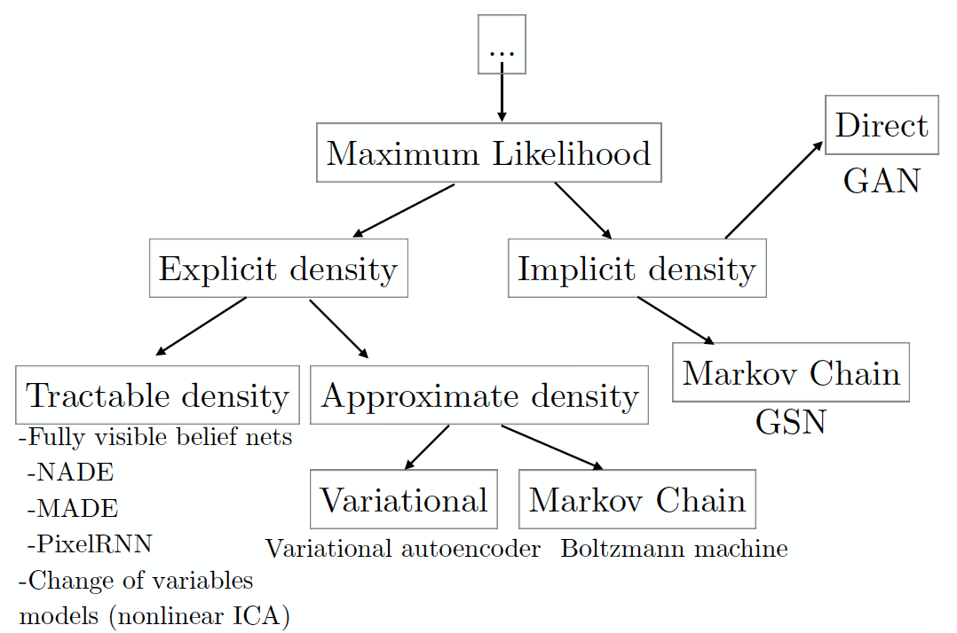
(the image is taken from the article by the author GANs, which is compiled on the basis of his seminar at the NIPS 2016 conference; from the same place there is a free retelling in several paragraphs below).
Recall that the essence of the maximum likelihood principle is to search for such model parameters that maximize the likelihood of a data set consisting of examples selected independently from the general population: . Usually, for ease of calculation, the likelihood logarithm is maximized:
Maximizing the likelihood is the same as minimizing the KL divergence between the present data distribution and the model:
Each leaf of the taxonomy tree corresponds to a specific model, which has a number of pros and cons. The GANs were developed with the aim of leveling the deficiencies of other models, which naturally led to the emergence of new deficiencies. But first things first. In the left subtree are models with explicitly defined form of the data density function. ( explicit density ). For such models, maximization is quite obvious, you need to insert the required density form into the likelihood logarithm formula and use the gradient lift to find the best set of parameters . The main disadvantage of this approach is the need to explicitly express the density so as to describe the whole variety of simulated data, but at the same time so that the resulting optimization problem can be solved in a reasonable time. If you manage to design everything so that the distribution satisfactorily describes the whole variety of data, and one of the models of the tractable density group works in a reasonable time, then consider yourself lucky (for now, by the way, the only way to assess the quality of the generated images is through human visual assessment).
If the model creates images of mediocre quality, or you have grown old while she was studying, then perhaps models that approximate density will solve the problem (see the sheet for approximate density ). Such models still need to provide an explicit density distribution formula. Methods based on variational approximation ( variational ) maximize the lower likelihood estimate , which guarantees the receipt of such an assessment of the real likelihood, which is at least as good as that obtained. For many noncomputable distributions, it is possible to find lower bounds that are computable in a reasonable time.
The main disadvantage of such models is that the gap between the lower estimate and the real credibility may be too great. This will result in the fact that the model learn something different but not real data distribution . If you are faced with this problem, then there is still the last chance for a successful approximation of the density you specified - the Monte Carlo methods ( Markov Chain Monte Carlo , MCMC), i.e. sampling. Sampling is the main drawback of this class of models. Despite the fact that the framework ensures that someday the sample will converge to This process may take an unacceptable amount of time.
Out of desperation, you can decide to use models with an implicit density function ( Implicit density ) - models that do not directly formulate , but only samples from it. Here we find ourselves either in the conditions of the previous method, when it is necessary to use Monte-Carlo methods for sampling with all the consequences, or you can use GANs, which generate one sample in one pass (which is comparable to one step of the Markov chain). So, to summarize, with what Ghana are so remarkable:
- they do not require explicit density, although it is possible to make sure that the desired form of distribution is learned (in this sense, variational methods and GANs are related);
- the derivation of the lower likelihood logarithm estimate is not required;
- no need to sample (more precisely, sampling is, but only in one step, not a chain);
- it was noticed that the images are better than those of other models (subjective assessment, of course);
- I'd add that this model is one of the easiest to understand in all the above categorization.
Naturally, everything is not so rosy, and in the subsequent parts of the analysis of GANs we will learn about all the new problems that have appeared along with the new model. Let's start with the very first article, in which the GANs were presented to the general public.
Generative Adversarial Networks (10 Jun 2014)
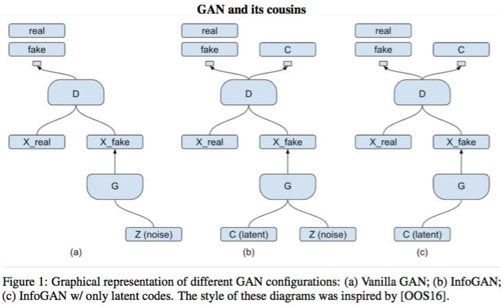
Imagine a story from a film about the counterfeiter's and the police confrontation: one forges, the other catches, you understand. What happens if we replace both of them with a neural network? Get a role-playing game, while only two actors.  G enerator is an analog of a counterfeiter, a network that generates data (for example, images), its task is to be able to produce images that are closest to the target population. D iscriminator - an analogue of a policeman, more precisely, that officer of the analytical department of the police in the fight against counterfeiters; His task is to distinguish the original coin from a fake. Thus, the discriminator is nothing more than a binary classifier, which must produce 1 for real images, and 0 for fake. Here it is worth remembering the Chinese room : what if the optimal discriminator cannot distinguish a fake from a real one, can we assume that the generator began to generate real images, or is it still a high-quality fake? In general, the model looks as follows and is trained by the end-to-end method of back propagation of an error:
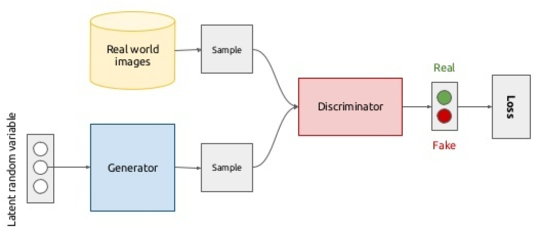
In principle, with the script in the upper half of the diagram, everything is clear: let's sample the images from the database of real images ( ), we assign the label 1 to them and run through the discriminator, so we get the probabilities of belonging to the class of real images. Maximizing the discriminator's log-likelihood on a sample of real and generated (more on this later) images, we move the density in the direction of real images: where - neural network discriminator, and - its parameters. For generator training, we denote the generator distribution as where - this is an image. Some prior noise distribution is introduced. which is displayed in the image space by the generator: ( - parameters of the network-generator). Yes, you understood everything correctly, images will be generated from noise. Moreover, we have the ability to customize the shape of this noise. In the second scenario, the following functionality is minimized: i.e. we want the discriminator to distinguish fake from real images as badly as possible. Nothing prevents us from updating the generator weights with a gradient descent, since - differentiable function. Combining all of the above into one optimization task, we get the following minimax game for two players:
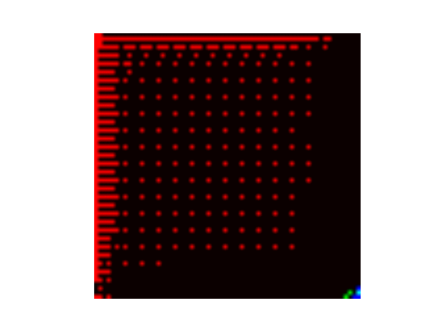
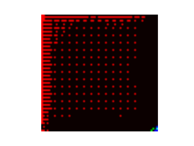
You may notice that this is very similar to the initial learning conditions with reinforcement, and you will be right. The channel of information transfer from the generator to the discriminator is a direct pass through the network, and the reverse pass is a method of transmitting information from the discriminator to the generator. The idea is to train the entire end-to-end model, simply inverting the gradients that come from the discriminator, which will allow the discriminator to climb higher on its surface, and the generator to descend on its own (see the next part, where the authors introduce the gradient reversal layer). But for GANs, this approach does not work. At the very beginning of learning, it is very easy for a discriminator to distinguish a fake from real data (see the example below). Then for fake data , and , which is expressed in the attenuation of the gradients. Simply put, no information from the discriminator will reach the generator, and the generator will lose (it will not learn anything). Assuming that the discriminator will always be near the optimum, replacing on solve the problem of attenuation, but the solution of the minimax game and the new maxmax one will be the same.
Compare what samples the network produces at the beginning of training and at a later stage.
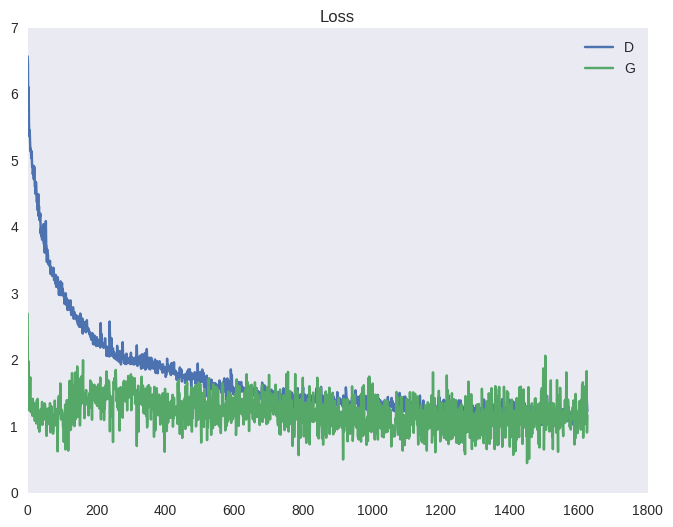
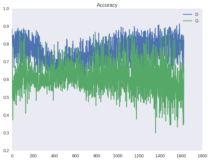
To ensure that the discriminator is always near the optimum, the authors of the article offer the following trick. At each iteration of training, first a few steps the discriminator learns in batches from real and fake images with a fixed generator; then one step is taken of learning the generator on a batch of fake images with a fixed discriminator. This will keep the discriminator always near the optimum and slowly change the generator. The result is a game of tug-of-war, which translates into unstable training. Below is a typical picture for the cost function of the GAN and for accuracy (average between the number of examples that the discriminator recognizes correctly in its training phase and in the training phase of the generator). You can observe the effect of such dragging on the graphs below, as well as in the form of ripples in the examples above (under the spoiler).
 |  |

Let's evaluate what theoretical rationales underlie GANs. First, the authors prove that for a fixed generator the optimal discriminator looks like:
And then they prove the theorem on the existence of a global minimum of the functional of the generator function at the point and also that the value of the function . Finally, the authors prove that the process of sequential learning of the generator and the discriminator converges. Everything seems to be very good, but all these calculations are true only if we consider all possible functions as candidates for the generator and discriminator. Unfortunately, in reality, we cannot solve the optimization problem in the space of all functions, and we have to restrict ourselves to a single family. In this case, this is a family of neural networks, i.e. parametrically defined functions. And that's just the reason for this unstable behavior, shown in the graphs above. By optimizing the functional in the space of parameters of neural networks (and this is the space of real numbers of very high dimension), we are simply unable to find the same global optimum. Why neural networks? For neural networks, the universal approximation theorem is proved, and, probably, this is still the widest class of functions in whose space we are able to search for a solution.
In conclusion of the review of the main article, let us consider the idealized visualization of the convergence process and what it leads to:

- black dotted is data distribution which we want to bring neural network;
- the green line is the generator distribution In the process of learning, it approaches the distribution of data (learning takes place sequentially);
- the blue line is the separating surface of the discriminator, which at the end of the training cannot distinguish examples from the actual data set from the forgery created by the generator;
- arrows show mapping which sets in correspondence to each value from the data distribution a point from the a priori distribution.
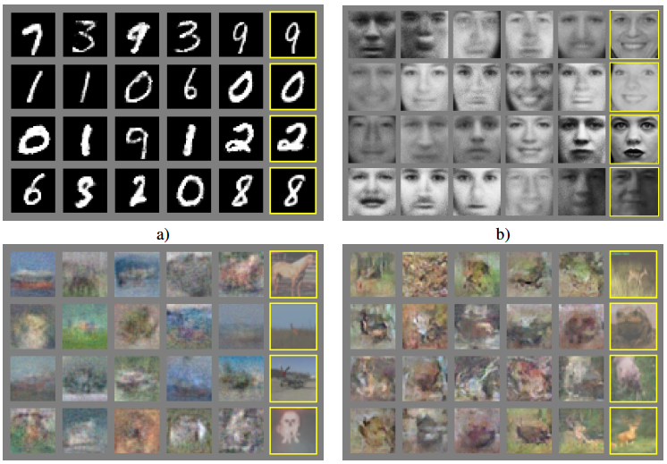
The authors present the results of four experiments. In the first five columns there are several samples from the generator, and on the right are the closest real images. Due to the use of MLP , the results on complex data sets are not yet impressive.
We note four properties of such training:
- it turns out that a smooth and compact space is learned (not to be confused with mathematical concepts), such that prototypes of similar objects in the noise space also lie next to each other (the authors use the ordinary MLP , because we will see beautiful visualizations in one of the following articles where convolutional networks), and for any point of a priori noise there is a meaningful preimage;
- the generator learns to create close-to-real images, never seeing a single real image, but only receiving a signal from the discriminator about why the fake was detected, encoded in gradients;
- kind of like trying to get rid of MCMC , because it takes a lot of time, but in the end they got a model that makes sampling in one step, but it still learns long and unstable (MCMC at least asymptotically converges, and here there are no guarantees in the space of parametric functions);
- the model is beautiful, but not at all applicable for extracting features from the image, which is what we ultimately need, because we want to not only generate, but also calculate the inverse images of real images in the noise space.
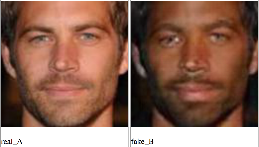
Unsupervised Domain Adaptation by Backpropagation (Sep 26, 2014)
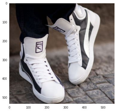
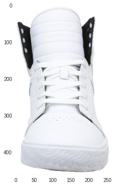
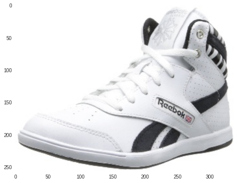
It seemed to everyone that Ghana was fun and provocatively, but for now it is useless. While humankind was aware of how to adapt them for the extraction of traits, an unexpected and useful application to GANs was found in Skolkovo. Imagine the following task: you need to do a search for clothes on real life photos in an Amazon-type store. To do this, we can easily collect the marked dataset, simply by sparking Amazon. Then assign a label to each image by product category, train the classifier and use some kind of network representation to search. But there is a small problem: all photos on Amazon, as a rule, are studio photos with a white background, no noise, and often no people at all. , , . , , , , , .
Domain Shift – , . , ; , ; , , . , , . - .
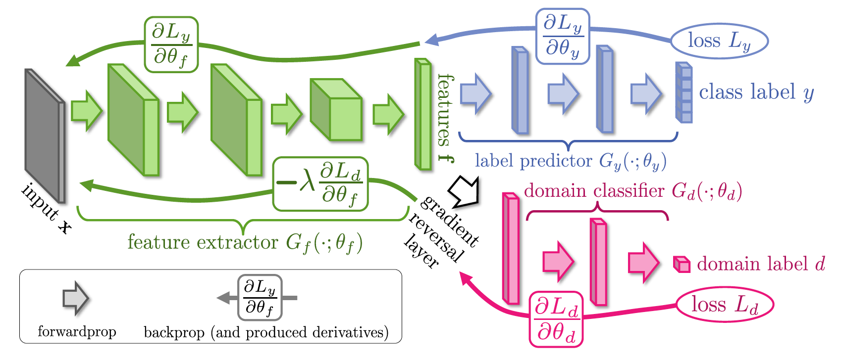
, , f , , Google Inception V1 , , . "" f , "" , .. . , end-to-end, gradient reversal layer, f . , f , , .
Target Photo:
Top 3 Answers:
Conditional Generative Adversarial Nets (6 Nov 2014)
, . , , , , .
, . . , MNIST, . , . MNIST, , , .
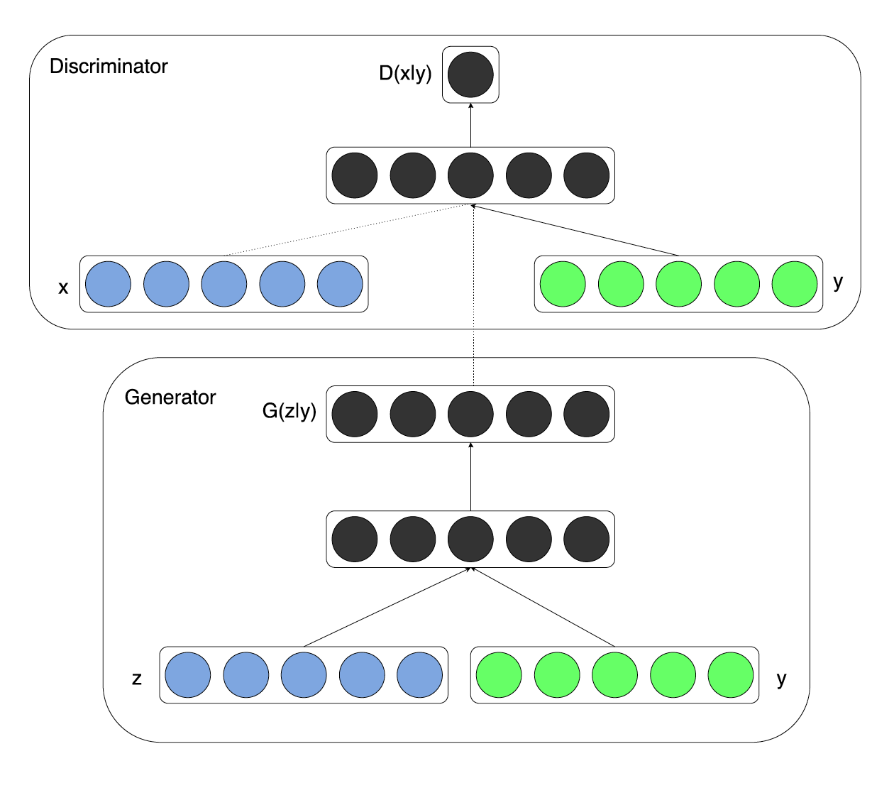
:
As a result, the authors hope, there will be a disentanglement of factors of the fashion and other parameters of the object. In the case of handwritten numbers, there is a funny effect: the model is no longer required to encode information about the label (number) into the feature vector (into the input noise), since all the information is already in the tag vector , then in the feature vector encoded information about the style of writing numbers. Each line in the next image is samples from the same mode (fixed tag vector).

Unsupervised Representation Learning with Deep Convolutional Generative Adversarial Networks (9 Nov 2015)
This article has more practical value than theoretical. Even the authors themselves note that the main contribution of the article is as follows:
- the usual neural network has been replaced by a convolutional one, and as a result of trial and error, instructions have been made on how to train D eep C onvolutional GAN ;
- It is shown in the examples that the discriminator obtained during the DCGAN training is a good initialization for other classifiers on this and similar domains (transfer learning to a learning task with a teacher from a learning task without a teacher);
- After analyzing the filters, the authors showed that it is possible to find filters that are responsible for drawing a specific object;
- It is shown that the generator has interesting properties similar to word2vec (see the example below).
Actually, there is nothing unexpected in the model itself, and, probably, experiments on training the model took just a lot of time - more than a year passed between the article on GANs and DCGAN (yet, of course, the authors played their part precisely because ICLR 2016 ). Here is the generator circuit:
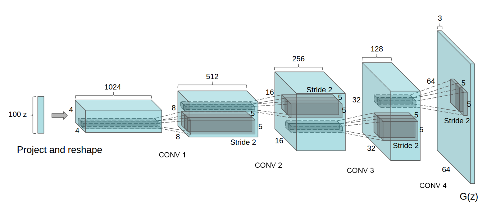
The features of the architecture include the following points:
- in the generator and discriminator instead of pooling, convolutions are used with a step greater than one (stride and fractional stride, respectively);
- batch normalization is used in the generator and the discriminator;
- full connected layers are not used, i.e. the network becomes fully convolutional;
- in the generator, everywhere, except for the output layer, ReLU is used (in the output layer - tanh);
- in the discriminator, Leaky ReLU is used everywhere.
As a result, we can enjoy creeping faces and arithmetic over them. More specifically, arithmetic is done in the feature space, and then the result is generated from the resulting vector.

')
We should also mention the details of the experiment itself. To begin with, they had to assemble a bunch of images, then find there with their hands and eyes a number of images of men with glasses, men without glasses, and women without glasses. Then the feature vectors of each group are averaged, arithmetic is done, and a new image is generated from the resulting feature vector.
In the description of the first article I wrote that the feature space is smooth and compact, i.e. if you choose a random point that lies on a variety of data prototypes, then around this point in all directions there will be signs whose images are similar to the current one. Now you can randomly select several points in the feature space, then start sampling the points along the path connecting the samples, drawing for each sample its image in the image space (yes, there is an extra arrow there).
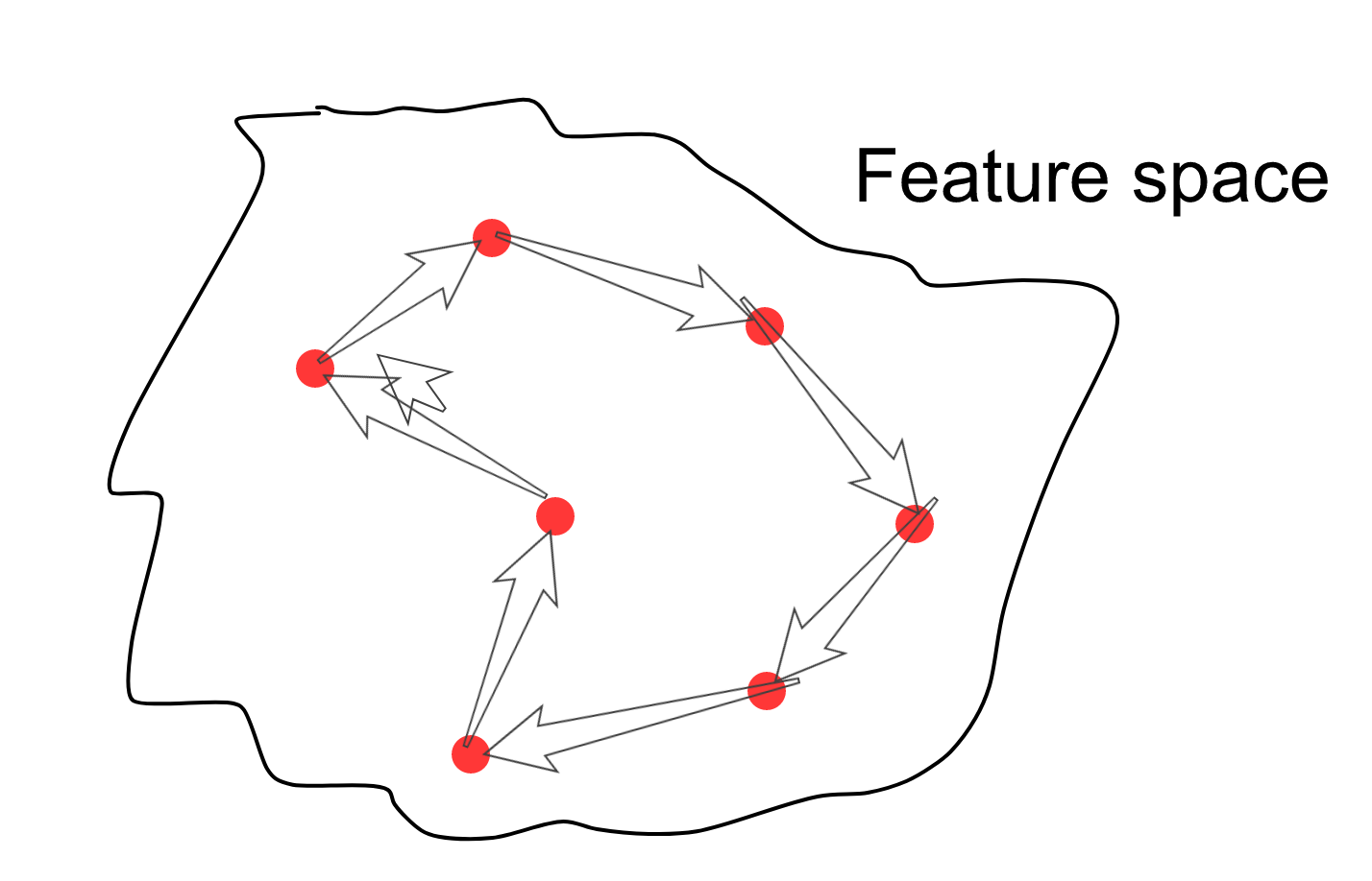
As a result, there will be such transitions of some creep faces to others.
In general, while in GANs, there is clearly not enough mechanism for extracting features from images. And here we come to the second most important article after the original article about GANs - "Adversarial Autoencoders".
Adversarial Autoencoders (Nov 18 2015)
The second most important article in GANs appeared a year and a half later after the original article, which is again due to adjust to ICLR 2016. In this article, the authors essentially unwrap the original and useless GAN inside out and add another cost function, as in Google Inception V1 . The result is a special type of autoencoders - a model with which you can extract features from objects. Consider the topology of the AAE model and then pay attention to some properties of features of such an auto-encoder.

At the top of the image is the usual autoencoder. Denote the distribution generated by the encoder (encoder) as where taken from data distribution (napimer from the set of handwritten numbers MNIST). Accordingly, the decoder where is taken from the full (marginal) distribution of the hidden layer of the autoencoder. At the output of the decoder is the usual cost function of the auto-encoder, which brings the output of their decoder to the input to the encoder.
At the bottom left is the sample generator from some prior noise distribution. This can be either a given analytically distribution of the type of multidimensional normal, or a distribution of an unknown nature, some black box. We do not yet understand exactly how it works, but we can sample from it. Denote the prior distribution of the hidden layer as . The GAN-discriminator is attached to the hidden layer, in the lower part of the image on the right. The task of the discriminator is to distinguish examples from the prior distribution of attributes. and examples from the distribution generated by the encoder . In the process of learning such a competitive autoencoder, the discriminator modifies the encoder parameters with its gradients so that was approaching distribution . In this way, the coder learns the implicit prior distribution, or they say that it is given implicit prior, which is coded inside the network, but we cannot get its form analytically.
The result is an autoencoder with two cost functions: normal for data quality and GAN for the quality of the hidden layer. The model is trained by a stochastic gradient descent according to the following scenario:
- recovery phase: the usual iteration of autoencade learning, during which the encoder and decoder parameters are updated to minimize the image recovery error;
- regularization phase: iteration of the encoder update and discriminator. It, in turn, consists of two phases described in the learning scenario of ordinary GANs, i.e. You must first take a few steps of learning the discriminator on the batch of real and fake examples with a fixed generator, then take one step of learning the generator on the batch of fake images with a fixed discriminator.
After such training, we can hope that the network will learn to display images from the data space on the distribution specified by us, as well as to find an adequate image in the observation space for any point from the specified distribution above the code.
At the very beginning of the post there is a tree of taxonomy of generative models, pay attention to the variational autoencoder (VAE), which approximates the explicitly specified distribution of the hidden layer. VAE minimizes the upper bound of the negative log likelihood data:
Translating into Russian, the cost function contains both a recovery error and a penalty for the fact that the distribution of the output of the encoder differs from the given a priori . The second two terms in the last line are the regularizer so that the distribution on the hidden layer is of a certain shape. Without a regularizer, this would be an ordinary autoencoder. In AAE, instead of a KL regularization containing an explicitly specified distribution, the GAN is used, which penalizes for the empirical discrepancy of samples from the hidden layer to the distribution specified by some sampler. I remind you that this some sampler can be both an explicitly specified distribution and an empirical one.

In this image, the authors compare how examples are placed on hidden space using AAE and VAE. In the first line, the hidden space is a two-dimensional Gaussian, and the second line is a mixture of ten Gaussians. On the right, the authors sample the points from the hidden space and draw the corresponding images of handwritten numbers, as we see everything is really compact and smooth.
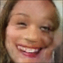
Also in this article describes some more perverted models based on AAE, which will form the basis of many other models in the future.
The model is very similar to the Conditional GAN, but also turned inside out. In the central part of the autoencoder is a hidden view composed of two vectors. The first displays the probability distribution of class membership. The second one displays a certain representation of the style (what else can remain if the figure itself is removed from writing the number). In the upper part there is a GAN part for class representation, which tries to bring the distribution above the classes given by the encoder (generator) to the real one-hot-encoding of this figure. The lower GAN tries to press information about the style into any distribution (in this case, in Gaussians). As a result, the class and style information is disentangled. For example, you can fix a class and generate a digit with different styles. Or vice versa, we fix the style and draw different numbers. It is worth noting that in the article they do not give such examples, but in the next article of this analysis this experiment is quite successful.
Such a model is useful if you have a certain number of marked examples and a much larger number of unlabeled (as often happens). Then for examples without a label, the upper GAN is not used.
After this article, astrologers have announced several years of GANs. In general, all articles after AAE can be divided into more engineering and more theoretical. The former tend to exploit different topologies, similar to the disentangling of styles in AAE. The latter concentrate more on the theoretical features of the GANs. We will consider several theoretical and several engineering articles. For those who decide to do practical implementation, it will be very useful to take a look at the article by the author GAN, based on his GAN tutorial at the NIPS conference in 2016: Improved Techniques for Training GANs .
InfoGAN: Generation Adversarial Nets Interpretable Representation Learning by Information (12 Jun 2016)
This article is a representative of a theoretical group of articles, in which the authors add to the learning process some informational and theoretical limitations, thus the hidden factors are better unraveled. The authors report on the successful unraveling of the style and written characters, the background of images from the object of interest, as well as hairstyles, emotions, and the fact that there are points on the dataset from the selfie. The authors also claim that the obtained signs in the mode of training without a teacher are comparable in quality with the signs obtained by training with a teacher. The authors do not forget to mention that generative models are the dominant type of models in the field of education without a teacher and remind that the ability to create objects entails a complete understanding of the structure of the object and, as a consequence, improved disentangling of factors.
In short, all these charms are achieved by maximizing the mutual information between observations and a certain subset of features from the internal representation of the autoencoder. Conventional GANs do not impose restrictions on the vector of the hidden representation, thus, in theory, the generator can begin to use factors in a very non-linear or related, thus none of the factors will be responsible for any semantic feature (remember the eigenfaces ). Before going into the details of InfoGAN, let me remind you of the objective function from the original GAN:
The model topology is identical to the model described in the Conditional GAN, the hidden layer is divided into two parts: - unavoidable noise, - vector containing semantic information about the object. We believe that latent factors are independent: . The generator of the new model can be written as . In ordinary GAN, the generator is not limited to ignoring semantic code. and may well come to a decision may not come. We would very much like it not to come, so the authors suggest adding an information-theoretical regularizer to the cost function. The idea of the regularizer is to maximize the mutual information between the semantic part of the hidden view and the generator distribution: .
Recall what mutual information is. Consider two random variables. and mutual information:
measures the "amount of information" obtained about the variable subject to variable observation . In other words, mutual information reflects the change in the uncertainty of the first variable when observing the second. If the mutual information is zero, then the second variable does not contain any information about the first variable. In our case, the more , the more information about the hidden layer is contained in the generated image. Otherwise, the image would completely ignore the semantic vector and would depend only on the noise vector, as in the original GAN. It turns out that for the generated example entropy will be smaller (see the second formula in the definition of mutual information), which can be reformulated as follows: in the process of generation, information about the semantic layer is not lost. Thus, the new cost function of such a cunning GAN, which can now be called InfoGAN, will be as follows:
But, unfortunately, this optimization problem becomes non-trivial due to the fact that we now need a posteriori distribution . And here comes the magic of variational output. For brevity, we denote , then:
KL-divergence is not negative, and the entropy of the hidden semantic layer can be considered constant, then the lower variational boundary of mutual information is obtained. By optimizing the lower bound, we optimize the value of the function itself, although the gap between the estimate and the real value is determined by the divergence and entropy. And, naturally, the distribution will be a neural network. It turns out that you need to add another discriminator to the model that will recognize the hidden vector fed into the generator. All this magic with variational reciprocal information resulted in another neural network. The authors advise fumbling the convolutional layers of the two discriminators, and only make a few fully connected layers at the output. InfoGAN will have the following topology:
Thus, the discriminator performs two functions: recognition of a real example from a false one and recovery of the vector of factors (or tags). When the present example is supplied without a label, the network recognizing the hidden semantic representation is simply not used. It may seem that InfoGAN is the same as the usual GAN, i.e. does not allow to extract features, but you can consolidate the material you read by trying to redo InfoGAN into the similarity of AAE.
In the MNIST experiment, a base of ten handwritten numbers, one categorical variable is used as a hidden layer as a semantic description and two noise .
Each column contains samples with a fixed category, but with a random noise component. Every line is the opposite. On the left, the results of InfoGAN show that the semantic variable contains information about the label (remember, labels did not participate in the training). On the right is the usual GAN and no interpretation.

And here, in each line, two of three hidden variables are fixed, all samples from InfoGAN. On the left, we fix the category and the second noise variable, on the right, the category and the first noise variable, and as a result we see that there is information about the style in the noise component.

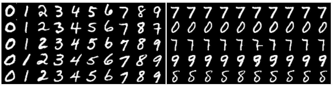
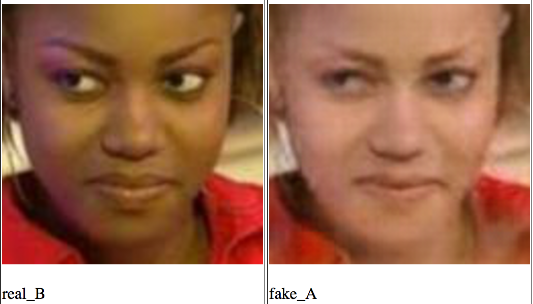
Unsupervised Cross-Domain Image Generation (7 Nov 2016)
Let us now consider an article that is more engineering than theoretical. By engineering, I mean a way to build a model that uses “mechanisms” (you need to cross the river — we build a bridge). Theoretical (in my notation) are models where a mathematical trick allows you to achieve a goal. . , S ource T arget, , . , . , , . , -: , S T T. Domain Transfer Network. , , . , . - , , .. . , , MSE. perceptual loss, style transfer .
, , . , Adversarial Autoencoder f-constancy loss, , AAE :
. , , - .
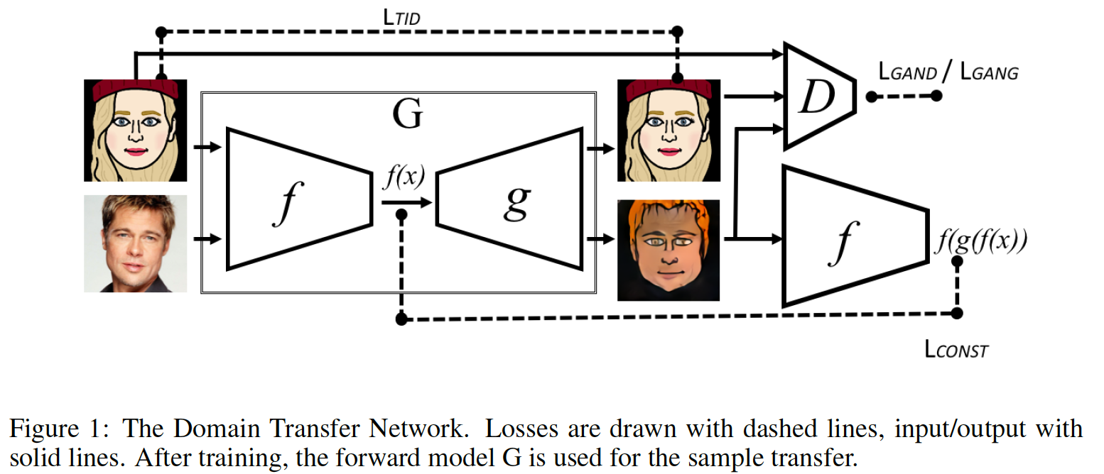
Generator , .. - : . .
, :
- T
- S
- T
:
- T , -
- f-constancy loss, S
- T ,
- total variation loss , —
- , DeepFace. http://bitmoji.com/ , , ( Facebook ). , , : ( ); , , ( ); — .
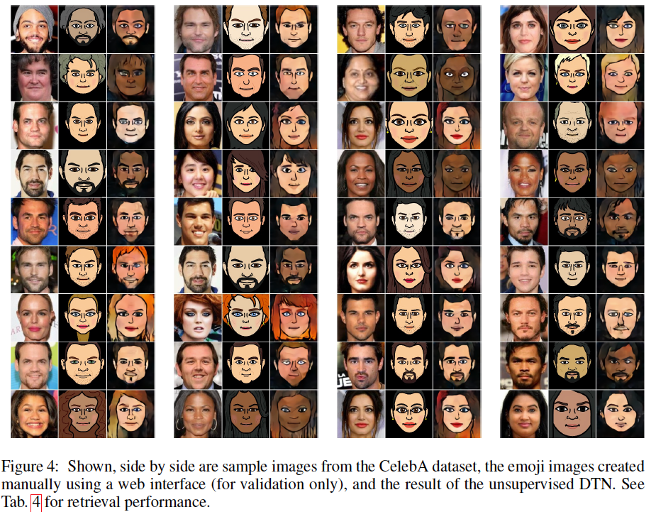
- :wat:
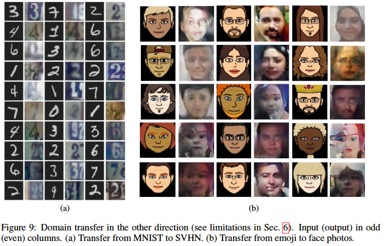
, . , FB . (, , 100 , , , ). , - "" .
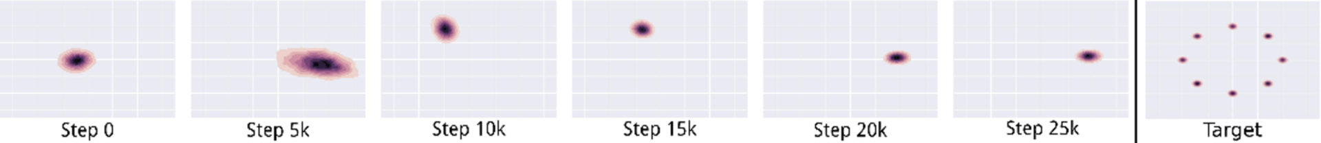
Unrolled Generative Adversarial Networks (7 Nov 2016)
. , , . , . , , : . , . , .. , . , , . Probably. "" — , . , and respectively. :
:
:
( ) ( ), :
, ( ), , . - - :
, . , , - , . , , , , . :
, ( ); , , , , . , .
, .. . . , . , , . , . (.. , ), , , . , , . , , , . , , ( ), .

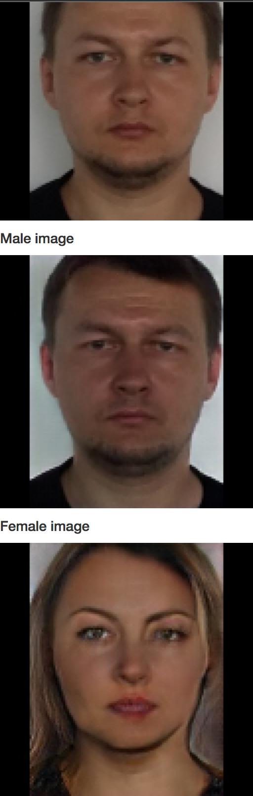
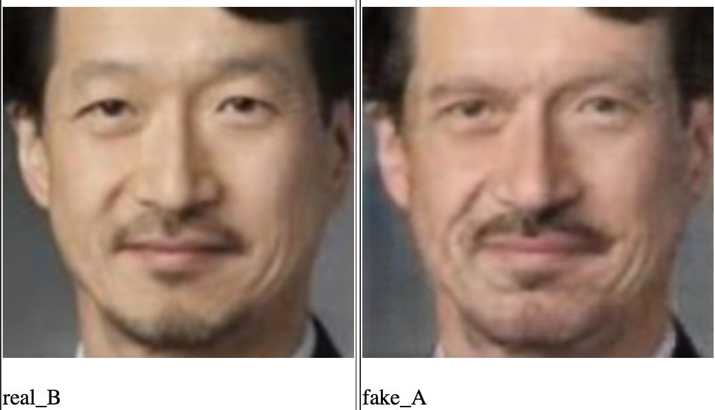
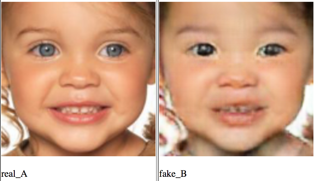
Unpaired Image-to-Image Translation using Cycle-Consistent Adversarial Networks (30 Mar 2017)
, , . .
, X Y, , . , , .
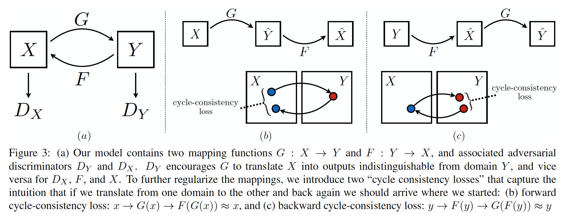
- and , , , (, ), . , , , , , . ( , , — ):
 |  |
PS: , , consistency loss , VGG , style transfer.
, .
Conclusion
. . , , :
- https://github.com/zhangqianhui/AdversarialNetsPapers
- https://github.com/nightrome/really-awesome-gan
- https://github.com/wiseodd/generative-models
- MIT .
- and for those adepts who understand reinforced learning, an article about the relationship between Ghana and reinforcement learning may be interesting.
It would be in general in life everything is as simple as in the GANs:
Thank you for the edits and advice to the following ladies and gentlemen from the datasetology lodge: bauchgefuehl , barmaley_exe , yorko , ternaus and movchan74 .
Source: https://habr.com/ru/post/322514/
All Articles