How to conduct A / B testing on Twitch

Experiments are one of the central functions of the scientific division of the Twitch streaming video site. We work closely with product managers to test new ideas and features. In the past, we used our own tools for conducting A / B experiments on the network and on our mobile applications. Recently, we tried a new approach to experiment on our Android application, using the phased deployment feature from Google Play.

Phased deployment allows developers to release a new build to a subset of the user base. Instead of implementing A / B logic within the application itself, developers, by introducing “if” blocks that support separate code processing and control paths, can create two separate versions and deploy them simultaneously. This feature is useful when making major changes in any application, for example, when redesigning the user interface. The negative side of phased deployments is the lack of control of the A / B ramifications for experiments. Phased deployment is usually used in the following cases:

1. Testing the sustainability of the new release;
2. Measuring the use of new features.

Since the new version of the application receives only a subset of users, this function is a great way to try out new ideas and roll them back if any problems occur. It also allows developers to measure the use of new features in an Android application. Twitch has an additional use case:
')
3. Measuring the impact of a new release on existing features

We would like to use phased deployments to measure the impact of new releases on an existing set of characteristics, such as, for example, daily active users. This feature is especially useful when making serious changes to some applications, where A / B logic is implemented for single binary file seems complicated.

Our initial approach was to use A / B testing with a phased deployment function. In this approach, the Google Play store selects a subset of users who are entitled to a test version of the application. Users who have received this right and updated - automatically or manually - the application to the new version, are marked as a test group. Users who have not upgraded to the new version are marked as a control group; This group may have users who have obtained the right to test version of the application, but have not installed the update. Users who switched to the new version only after a fixed time interval (in our experiment, 1 week) did not enter the experiment, since they covered both groups.

Google Play uses a randomized approach to select different groups of experiments, and we can measure key characteristics for these groups. However, we found data shifts that prevented our standard A / B testing from being applied.


The graph above shows the average number of daily sessions per active user for our test and control groups from a phased deployment. It can be seen that users with the new version of the application were more active than other users before the experiment, which meant a violation of the key A / B testing condition: a randomized sample should minimize the bias, leveling the impact of all other factors.

Since this condition was not met, it was necessary to use another way to measure the results of our experiments and bring them to our product managers. It was necessary to answer the following questions:

1. New release has a positive effect on our key features?
2. Is the change significant?
3. How big is the change?

Usually we compare the results obtained for the test and control groups for a certain time interval after the release of the experimental version. To determine changes in user groups with phased deployment, we measured the key characteristics of the experimental groups before and after the new release and compared the results of these groups. For the analysis two approaches were used:

1. Time series based analysis;
2. Estimation using the difference difference method.

We used the first approach to assess the absolute changes in key characteristics using the aggregated level data, and the second approach to test the significance of the set of characteristics using the user level data. Both approaches are used to calculate offsets in such a way that phased deployments represent users.

Phased Deployment Offsets

One of the problems known when using phased deployment on Google Play is that it may take several days for the user to update to the new binary release (APK). We used a selection rate of 10% for our test assembly, and it took users about 2 weeks to arrive at this value. The graph below shows the degree of acceptance of the new APK, where it refers to the ratio of the number of users who updated the version to the total number of active users.


We found that the inclusion of new users leads to a more rapid change in the degree of acceptance, but we have excluded these users from our analysis. Both methods — based on time series and “difference differences” - are based on data collected for each user before starting the experiment, and new users do not have such data. For the experiment described in detail in this article, we included only those users who switched to the new version within 1 week, which gave a degree of acceptance of 8.3%.

To try to explain the differences (offsets) in the data, we looked at the many variables that might be responsible for this. The following variables did not matter for group users:

1. A country;
2. Device model

Differences for groups showed such variables as the initial month for the user and the number of previous updates. The difference for users who have already performed updates was not surprising, since users had to have updates in order to be included in the test group.

Time Series Analysis

One of the characteristics measured in our phased deployment experiment was the average number of sessions per active user. To estimate the absolute value of the difference of this characteristic in the test and control groups, we used the CausalImpact R package, which performs Bayesian modeling based on time series. In this approach, an assessment of the time series of the test group occurs, if there is no disturbing influence, and this assessment is used to predict the relative and absolute changes in characteristics. The key condition of this approach is the absence of the effect of any changes being made on the control group.


The number of sessions for test and control (dashed) groups

The graphs at the top show the time dependencies for the test and control groups. The solid line represents the average number of sessions for the test group, which before the experiment exceeded that for the control group. We used the interval of two weeks before and after the release to measure key characteristics.

library(CausalImpact) data <- read.csv(data, file = "DailySessions.csv") #  DataFrame     ts <- cbind(data$test, data$control) matplot(ts, type = "l") #             pre.period <- c(1, 14) post.period <- c(15, 30) impact <- CausalImpact(ts, pre.period, post.period) #      plot(impact, c("original", "pointwise")) summary(impact, "report") 

We used the CausalImpact R package to assess the impact of the version of the new application on our session characteristics. The above code snippet shows how to use this package to build a test group assessment. In this experiment, the relative increase in the number of daily sessions per one active user was + 4% with a 95% confidence interval [+ 2%, + 5%].


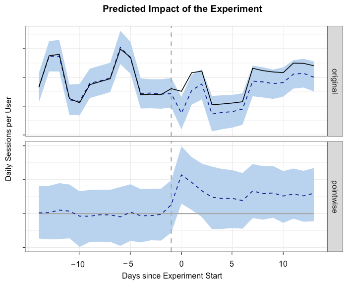
The predicted impact of the experiment

This approach is useful if there is only aggregated data. To figure out the effects of various variables regardless of the time component, we used bootstrapping.

Estimation using the difference difference method

When conducting experiments on Twitch, we usually track some set of characteristics. Bootstrapping is a powerful resampling process that allows our specialists to measure changes in performance at confidence intervals. In our phased deployment experiment, we used bootstrapping to measure the “difference of differences” between our test and control groups.

 library(boot) data <- read.csv("UserSessions.csv") #    " " run_DiD <- function(data, indices){ d <- data[indices,] new <- mean(d$postval[d$group=='Test'])/ mean(d$priorval[d$group=='Test']) old <-mean(d$postval[d$expgroup=='Control'])/ mean(d$priorval[d$expgroup=='Control']) return((new - old)/old * 100.0) } #      boot_est <- boot(data, run_DiD, R=1000, parallel="multicore", ncpus = 8) quantile(boot_est$t, c(0.025, 0.975)) plot(density(boot_est$t), xlab = "% Increase vs. Control") 

For each user, we measured the total number of sessions 14 days before the release of the test version and 14 days after the release. Then, on thousands of points, we calculated the average values ​​of the difference between the values ​​before and after the release of the version and determined the percentage difference between the test and control groups. For these calculations, we used the boot R package, as shown above. This model showed an increase of + 5.4% of the total number of sessions per user with a 95% confidence interval [+ 3.9%, + 6.9%].


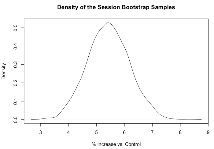
Density of sets of objects with repetitions of sessions

Summary

We found data differences when using the phased deployment feature of Google and applied new methods to experiment with this feature. Both approaches used showed that the new release of the application led to a marked increase in the number of sessions per user. The time series method is useful in cases where there is only aggregate level data, and the bootstrap approach is useful for testing different values ​​regardless of the time component. The phased deployment feature provides a mechanism for testing new builds, but it does not work with standard A / B testing approaches. Further information is available at Causal Impact and A / B Testing on Facebook.