Neural networks in pictures: from one neuron to deep architectures
Many materials on neural networks immediately begin with a demonstration of quite complex architectures. At the same time, the most basic things concerning the functions of activations, initialization of weights, selection of the number of layers in the network, etc. if considered, then passing. It turns out that a beginner of the practice of neural networks has to take typical configurations and work with them virtually blindly.
In the article we will go the other way. Let's start with the simplest configuration - one neuron with one input and one output, without activation. Next, in small iterations we will complicate the network configuration and try to squeeze a reasonable maximum out of each of them. This will allow you to pull the network for the strings and to gain practical intuition in building architectures of neural networks, which in practice turns out to be a very valuable asset.
Popular applications of neural networks, such as classification or regression, are a superstructure over the network itself, which includes two additional stages - preparation of input data (feature extraction, data conversion into vector) and interpretation of results. For our purposes, these additional stages are redundant, since we are not looking at the work of the network in its pure form, but at a certain construction, where the neural network is only an integral part.
')
Let's remember that the neural network is nothing but an approach to the approximation of the multidimensional function Rn -> Rn. Considering the limitations of human perception, in our article we will approximate the function on a plane. Several non-standard use of neural networks, but it is great for the purpose of illustration of their work.
To demonstrate the configurations and results, I suggest taking the popular framework Keras, written in Python. Although you can use any other tool for working with neural networks - most often the differences will be only in the names.
The simplest possible configuration of neural networks is one neuron with one input and one output without activation (or you can say with linear activation f (x) = x):

NB As you can see, two values are fed to the input of the network - x and one. The latter is necessary in order to introduce an offset b. In all popular frameworks, the input unit is already implicitly present and is not specified by the user separately. Therefore, hereinafter we will assume that one value is supplied to the input.
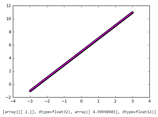
Despite its simplicity, this architecture already allows linear regression, i.e. approximate the function with a straight line (often with minimization of the standard deviation). The example is very important, so I propose to disassemble it in as much detail as possible.
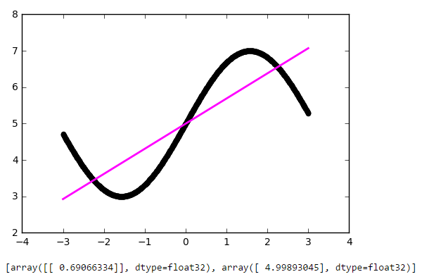
As you can see, our simplest network coped with the task of approximating a linear function with a linear function with a bang. Now let's try to complicate the task by taking a more complex function:
Again, the result is quite decent. Let's look at the weights of our model after training:
The first number is the weight w, the second is the offset b. To see this, let's draw the line f (x) = w * x + b:

It all fits together.
Well, as the line approaches, everything is clear. But this and the classical linear regression did quite well. How to capture the nonlinearity of the approximated function by the neural network?
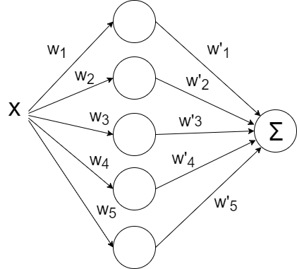
Let's try to throw in more neurons, let's say five pieces. Since one value is expected at the output, you will have to add one more layer to the network, which will simply summarize all the output values from each of the five neurons:
Run:
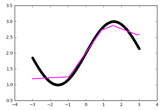
And ... nothing happened. All the same straight line, although the matrix weights has grown a bit. The fact is that the architecture of our network is reduced to a linear combination of linear functions:
f (x) = w1 '* (w1 * x + b1) + ... + w5' (w5 * x + b5) + b
Those. again is a linear function. To make the behavior of our network more interesting, we will add the function ReLU (rectifier, f (x) = max (0, x)) to the neurons of the inner layer, which allows the network to break the line into segments:
The maximum number of segments coincides with the number of neurons on the inner layer. By adding more neurons, you can get a more accurate approximation:
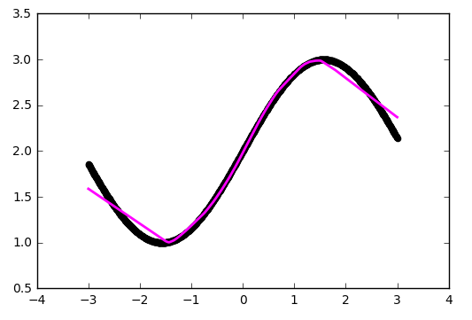
Already better, but flaws are visible to the eye - at the bends, where the original function is the least similar to a straight line, the approximation lags behind.
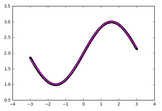
As an optimization strategy, we took a rather popular method - SGD (stochastic gradient descent). In practice, its improved version with inertia (SGDm, m - momentum) is often used. This allows you to more smoothly turn on sharp bends and the approximation becomes better by eye:
Sine is a pretty good feature for optimization. Mainly because it does not have wide plateaus - i.e. areas where the function changes very slowly. In addition, the function itself varies fairly evenly. To test our configuration for strength, take the function more complicated:
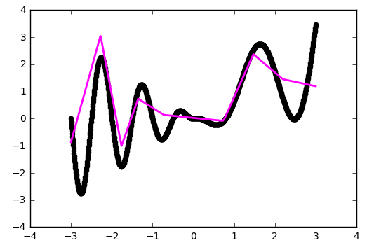
Alas, oh, here we already run into the ceiling of our architecture.
Let's try replacing the ReLU (rectifier) that served us in previous examples with a more non-linear hyperbolic tangent:
Approximation became better on the folds, but our network did not see part of the function. Let's try to play with one more parameter - the initial distribution of weights. We use the practical value of 'glorot_normal' (after the researcher Xavier Glorot, in some frameworks it is called XAVIER):
Already better. But using 'he_normal' (after the name of the researcher Kaiming He) gives an even more pleasant result:
Let's take a short pause and see how our current configuration works. A network is a linear combination of hyperbolic tangents:
f (x) = w1 '* tanh (w1 * x + b1) + ... + w5' * tanh (w5 * x + b5) + b
The illustration clearly shows that each hyperbolic tangent has captured a small area of responsibility and is working on approximating a function in its own small range. Outside its area, the tangent falls to zero or one and simply gives an offset along the ordinate axis.
Let's take a look at what is happening abroad in the network training area, in our case it is [-3, 3]
As was clear from the previous examples, beyond the boundaries of the learning area, all hyperbolic tangents turn into constants (strictly speaking, values close to zero or one). The neural network is not able to see outside the field of study: depending on the activators chosen, it will be very rude to estimate the value of the function being optimized. It is worth remembering this when constructing signs and inputs given for a neural network.
Until now, our configuration has not been an example of a deep neural network, since there was only one inner layer. Add one more:
You can see for yourself that the network has better worked out the problem areas in the center and near the lower border along the x-axis:
NB Blind adding layers does not automatically improve, which is called out of the box. For most practical applications, the two inner layers are quite sufficient, and you will not have to deal with the special effects of too deep networks, such as the problem of a vanishing gradient. If you do decide to go deep, be prepared to experiment a lot with network training.
Just put a little experiment:
From a certain point on, the addition of neurons to the inner layers does not give a gain in optimization. A good rule of thumb is to take the average between the number of inputs and outputs of the network.
Neural networks are a powerful, but non-trivial application tool. The best way to learn how to build working neural network configurations is to start with simpler models and experiment a lot by gaining experience and intuition in the practice of neural networks. And, of course, share the results of successful experiments with the community.
In the article we will go the other way. Let's start with the simplest configuration - one neuron with one input and one output, without activation. Next, in small iterations we will complicate the network configuration and try to squeeze a reasonable maximum out of each of them. This will allow you to pull the network for the strings and to gain practical intuition in building architectures of neural networks, which in practice turns out to be a very valuable asset.
Illustrative material
Popular applications of neural networks, such as classification or regression, are a superstructure over the network itself, which includes two additional stages - preparation of input data (feature extraction, data conversion into vector) and interpretation of results. For our purposes, these additional stages are redundant, since we are not looking at the work of the network in its pure form, but at a certain construction, where the neural network is only an integral part.
')
Let's remember that the neural network is nothing but an approach to the approximation of the multidimensional function Rn -> Rn. Considering the limitations of human perception, in our article we will approximate the function on a plane. Several non-standard use of neural networks, but it is great for the purpose of illustration of their work.
Framework
To demonstrate the configurations and results, I suggest taking the popular framework Keras, written in Python. Although you can use any other tool for working with neural networks - most often the differences will be only in the names.
The easiest neural network
The simplest possible configuration of neural networks is one neuron with one input and one output without activation (or you can say with linear activation f (x) = x):
NB As you can see, two values are fed to the input of the network - x and one. The latter is necessary in order to introduce an offset b. In all popular frameworks, the input unit is already implicitly present and is not specified by the user separately. Therefore, hereinafter we will assume that one value is supplied to the input.
Despite its simplicity, this architecture already allows linear regression, i.e. approximate the function with a straight line (often with minimization of the standard deviation). The example is very important, so I propose to disassemble it in as much detail as possible.
import matplotlib.pyplot as plt import numpy as np # -3 3 x = np.linspace(-3, 3, 1000).reshape(-1, 1) # , def f(x): return 2 * x + 5 f = np.vectorize(f) # y = f(x) # , Keras from keras.models import Sequential from keras.layers import Dense def baseline_model(): model = Sequential() model.add(Dense(1, input_dim=1, activation='linear')) model.compile(loss='mean_squared_error', optimizer='sgd') return model # model = baseline_model() model.fit(x, y, nb_epoch=100, verbose = 0) # plt.scatter(x, y, color='black', antialiased=True) plt.plot(x, model.predict(x), color='magenta', linewidth=2, antialiased=True) plt.show() # for layer in model.layers: weights = layer.get_weights() print(weights) As you can see, our simplest network coped with the task of approximating a linear function with a linear function with a bang. Now let's try to complicate the task by taking a more complex function:
def f(x): return 2 * np.sin(x) + 5 Again, the result is quite decent. Let's look at the weights of our model after training:
[array([[ 0.69066334]], dtype=float32), array([ 4.99893045], dtype=float32)] The first number is the weight w, the second is the offset b. To see this, let's draw the line f (x) = w * x + b:
def line(x): w = model.layers[0].get_weights()[0][0][0] b = model.layers[0].get_weights()[1][0] return w * x + b # plt.scatter(x, y, color='black', antialiased=True) plt.plot(x, model.predict(x), color='magenta', linewidth=3, antialiased=True) plt.plot(x, line(x), color='yellow', linewidth=1, antialiased=True) plt.show() It all fits together.
Let's complicate the example
Well, as the line approaches, everything is clear. But this and the classical linear regression did quite well. How to capture the nonlinearity of the approximated function by the neural network?
Let's try to throw in more neurons, let's say five pieces. Since one value is expected at the output, you will have to add one more layer to the network, which will simply summarize all the output values from each of the five neurons:
def baseline_model(): model = Sequential() model.add(Dense(5, input_dim=1, activation='linear')) model.add(Dense(1, input_dim=5, activation='linear')) model.compile(loss='mean_squared_error', optimizer='sgd') return model Run:
And ... nothing happened. All the same straight line, although the matrix weights has grown a bit. The fact is that the architecture of our network is reduced to a linear combination of linear functions:
f (x) = w1 '* (w1 * x + b1) + ... + w5' (w5 * x + b5) + b
Those. again is a linear function. To make the behavior of our network more interesting, we will add the function ReLU (rectifier, f (x) = max (0, x)) to the neurons of the inner layer, which allows the network to break the line into segments:
def baseline_model(): model = Sequential() model.add(Dense(5, input_dim=1, activation='relu')) model.add(Dense(1, input_dim=5, activation='linear')) model.compile(loss='mean_squared_error', optimizer='sgd') return model The maximum number of segments coincides with the number of neurons on the inner layer. By adding more neurons, you can get a more accurate approximation:
Give more accuracy!
Already better, but flaws are visible to the eye - at the bends, where the original function is the least similar to a straight line, the approximation lags behind.
As an optimization strategy, we took a rather popular method - SGD (stochastic gradient descent). In practice, its improved version with inertia (SGDm, m - momentum) is often used. This allows you to more smoothly turn on sharp bends and the approximation becomes better by eye:
# , Keras from keras.models import Sequential from keras.layers import Dense from keras.optimizers import SGD def baseline_model(): model = Sequential() model.add(Dense(100, input_dim=1, activation='relu')) model.add(Dense(1, input_dim=100, activation='linear')) sgd = SGD(lr=0.01, momentum=0.9, nesterov=True) model.compile(loss='mean_squared_error', optimizer=sgd) return model Complicate further
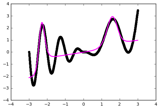
Sine is a pretty good feature for optimization. Mainly because it does not have wide plateaus - i.e. areas where the function changes very slowly. In addition, the function itself varies fairly evenly. To test our configuration for strength, take the function more complicated:
def f(x): return x * np.sin(x * 2 * np.pi) if x < 0 else -x * np.sin(x * np.pi) + np.exp(x / 2) - np.exp(0) Alas, oh, here we already run into the ceiling of our architecture.
Give more nonlinearity!
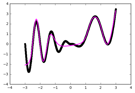
Let's try replacing the ReLU (rectifier) that served us in previous examples with a more non-linear hyperbolic tangent:
def baseline_model(): model = Sequential() model.add(Dense(20, input_dim=1, activation='tanh')) model.add(Dense(1, input_dim=20, activation='linear')) sgd = SGD(lr=0.01, momentum=0.9, nesterov=True) model.compile(loss='mean_squared_error', optimizer=sgd) return model # model = baseline_model() model.fit(x, y, nb_epoch=400, verbose = 0) Scale initialization is important!
Approximation became better on the folds, but our network did not see part of the function. Let's try to play with one more parameter - the initial distribution of weights. We use the practical value of 'glorot_normal' (after the researcher Xavier Glorot, in some frameworks it is called XAVIER):
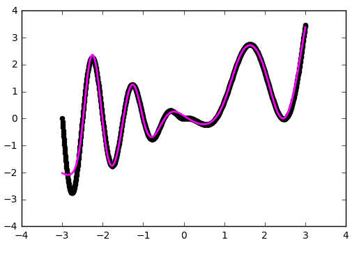
def baseline_model(): model = Sequential() model.add(Dense(20, input_dim=1, activation='tanh', init='glorot_normal')) model.add(Dense(1, input_dim=20, activation='linear', init='glorot_normal')) sgd = SGD(lr=0.01, momentum=0.9, nesterov=True) model.compile(loss='mean_squared_error', optimizer=sgd) return model Already better. But using 'he_normal' (after the name of the researcher Kaiming He) gives an even more pleasant result:
How it works?
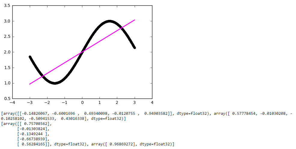
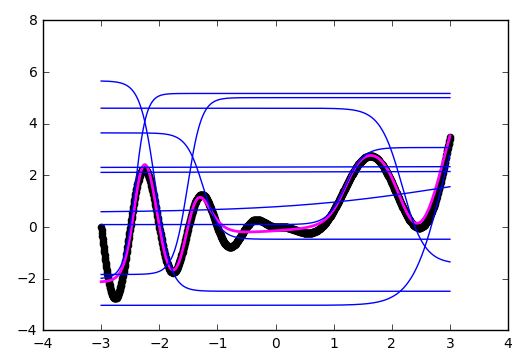
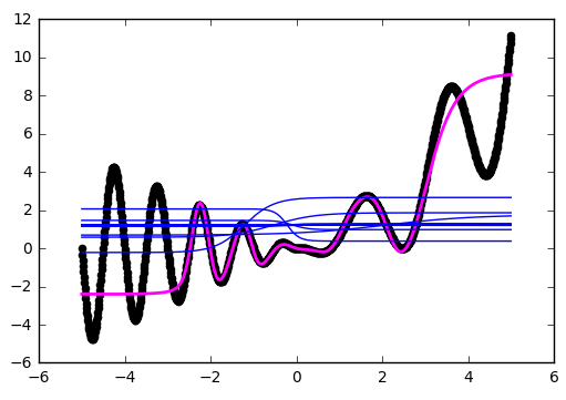
Let's take a short pause and see how our current configuration works. A network is a linear combination of hyperbolic tangents:
f (x) = w1 '* tanh (w1 * x + b1) + ... + w5' * tanh (w5 * x + b5) + b
# def tanh(x, i): w0 = model.layers[0].get_weights() w1 = model.layers[1].get_weights() return w1[0][i][0] * np.tanh(w0[0][0][i] * x + w0[1][i]) + w1[1][0] # plt.scatter(x, y, color='black', antialiased=True) plt.plot(x, model.predict(x), color='magenta', linewidth=2, antialiased=True) # for i in range(0, 10, 1): plt.plot(x, tanh(x, i), color='blue', linewidth=1) plt.show() The illustration clearly shows that each hyperbolic tangent has captured a small area of responsibility and is working on approximating a function in its own small range. Outside its area, the tangent falls to zero or one and simply gives an offset along the ordinate axis.
Abroad area of study
Let's take a look at what is happening abroad in the network training area, in our case it is [-3, 3]
As was clear from the previous examples, beyond the boundaries of the learning area, all hyperbolic tangents turn into constants (strictly speaking, values close to zero or one). The neural network is not able to see outside the field of study: depending on the activators chosen, it will be very rude to estimate the value of the function being optimized. It is worth remembering this when constructing signs and inputs given for a neural network.
Go into the depths
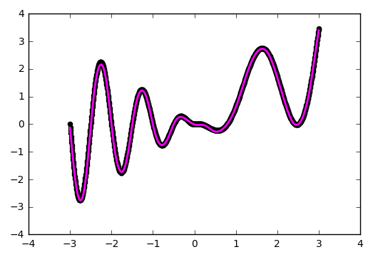
Until now, our configuration has not been an example of a deep neural network, since there was only one inner layer. Add one more:
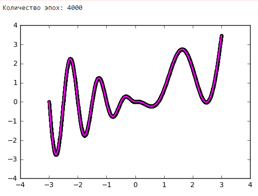
def baseline_model(): model = Sequential() model.add(Dense(50, input_dim=1, activation='tanh', init='he_normal')) model.add(Dense(50, input_dim=50, activation='tanh', init='he_normal')) model.add(Dense(1, input_dim=50, activation='linear', init='he_normal')) sgd = SGD(lr=0.01, momentum=0.9, nesterov=True) model.compile(loss='mean_squared_error', optimizer=sgd) return model You can see for yourself that the network has better worked out the problem areas in the center and near the lower border along the x-axis:
An example of working with one inner layer
NB Blind adding layers does not automatically improve, which is called out of the box. For most practical applications, the two inner layers are quite sufficient, and you will not have to deal with the special effects of too deep networks, such as the problem of a vanishing gradient. If you do decide to go deep, be prepared to experiment a lot with network training.
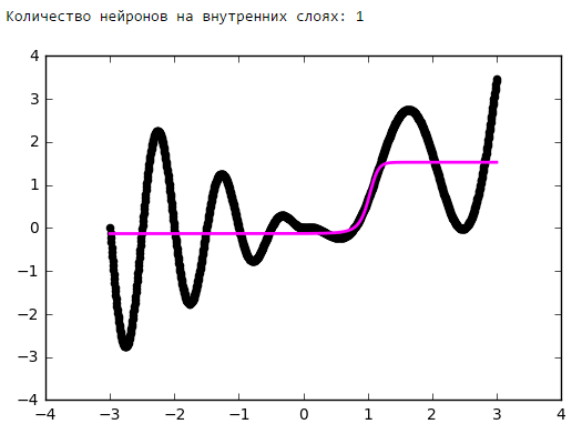
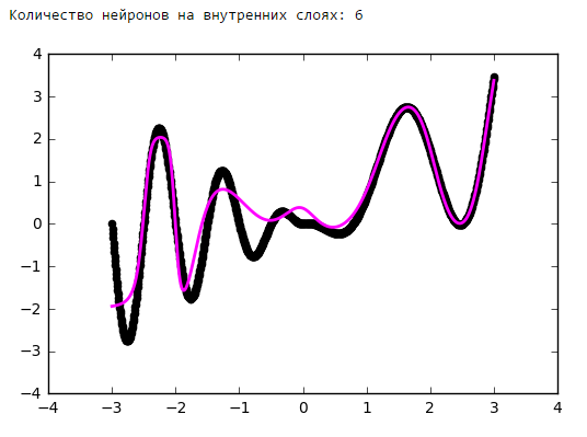
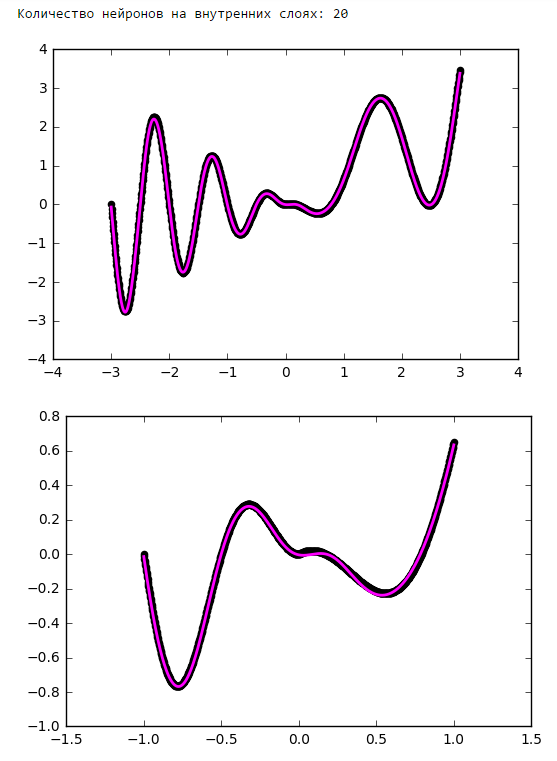
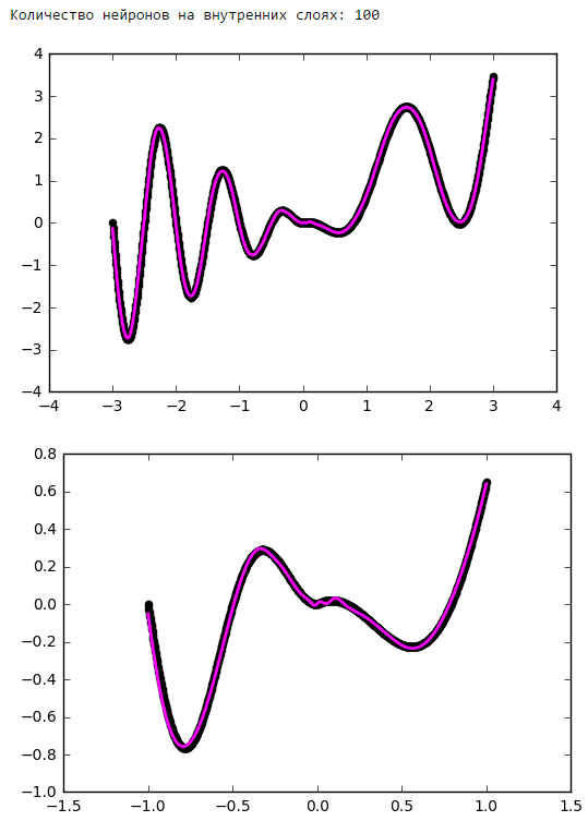
The number of neurons on the inner layers
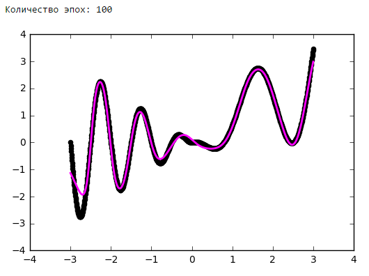
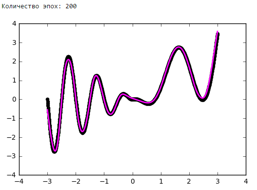
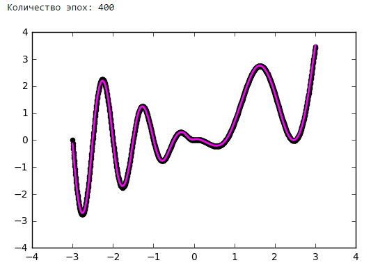
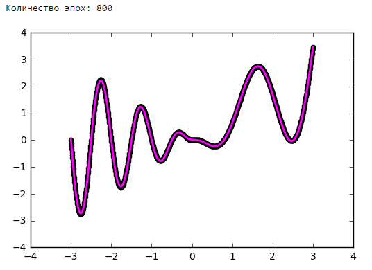
Just put a little experiment:
From a certain point on, the addition of neurons to the inner layers does not give a gain in optimization. A good rule of thumb is to take the average between the number of inputs and outputs of the network.
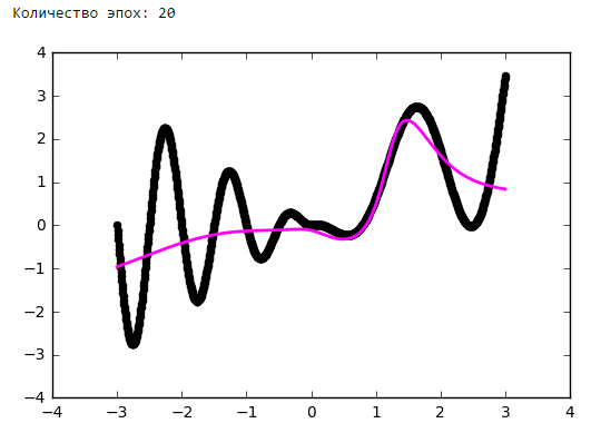
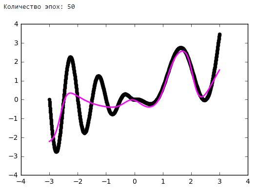
Number of epochs
findings
Neural networks are a powerful, but non-trivial application tool. The best way to learn how to build working neural network configurations is to start with simpler models and experiment a lot by gaining experience and intuition in the practice of neural networks. And, of course, share the results of successful experiments with the community.
Source: https://habr.com/ru/post/322438/
All Articles