Measurement of throughput of bottlenecks in time of double pass packet

By all measures, today's Internet cannot transfer data as quickly as it should. Most mobile users in the world experience delays from a few seconds to a few minutes: public WiFi points at airports and conferences are even worse. Physicists and climatologists need to share petabytes of data with colleagues around the world, but they are faced with the fact that their carefully designed multi-gigabit infrastructure often yields just a few megabits per second on transcontinental lines. [6]

These problems arose because of the choice of architecture that was made when creating the TCP congestion control system in the 1980s — then they decided to interpret the packet loss as a “jam”. [13] The equivalence of these concepts was fair for that time, but only because of the limitations of the technology, and not by definition. When NICs (network interface controllers) were upgraded from megabyte to gigabit speeds, and memory chips from kilobytes to gigabytes, the connection between packet loss and congestion became less obvious.

In today's TCP, congestion control for packet loss — even in the most advanced technology of this kind of CUBIC [11] —is the main cause of these problems. If bottlenecks are too large, the congestion control system for packet loss keeps them full, causing excessive network buffering. If the buffers are too small, then the congestion control system for packet loss incorrectly interprets packet loss as a congestion signal, which leads to a decrease in throughput. Solving these problems requires an alternative to congestion control for packet loss. To find this alternative, it is necessary to understand where and how congestion occurs.

Clogging and bottleneck

At any given time in a (full duplex) TCP connection there is only one slowest link or bottleneck in each direction. The bottleneck is important for the following reasons:
')

• It determines the maximum data transfer rate for the connection. This is the main property of an uncompressed data stream (for example, imagine a six-lane highway during rush hours if, due to accidents, one small segment of the road is limited to just one lane. The traffic in front of the crash site will move no faster than the traffic through this lane.
  
  
• This is the place where queues are constantly formed. They are reduced only if the intensity of the outflow from the bottleneck exceeds the intensity of the incoming stream. For connections operating at the maximum transfer rate, all outgoing flows to the bottleneck always have a higher outgoing flow rate, so the queues move to the bottleneck.

Regardless of how many links are in a connection and what their speeds are separately, from a TCP point of view, an arbitrarily complex route is represented as a single connection with the same RTT (time of double pass of a packet, i.e., round trip time) and throughput of the bottleneck . Two physical constraints, RTprop (round-trip propagation time, packet double pass time) and BtlBw (bottleneck bandwidth), affect transmission performance. (If the network path were a material pipe, RTprop would be a pipe length, and BtlBw would be its diameter).

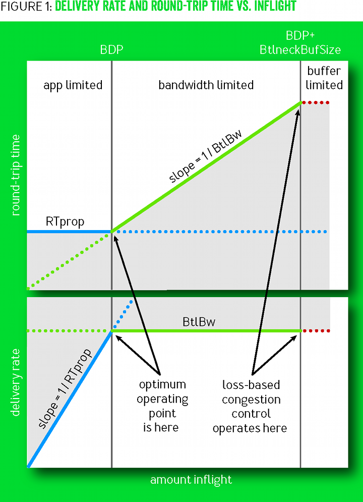
Figure 1 shows various combinations of RTTs and transfer rates with the amount of data in flight , that is, inflight (data sent, but without confirmation of delivery). The blue lines show the RTprop limit, the green lines show the BtlBw limit, and the red lines show the bottleneck buffer. Operations in gray areas are impossible, since they contradict at least one restriction. Transitions between the restrictions led to the formation of three regions (app-limited, bandwidth-limited and buffer-limited) with qualitatively different behavior.


Picture 1

When there is not enough data in flight to fill the tube, RTprop determines the behavior; otherwise, BtlBw dominates. Limit lines intersect at $$$inflight = BtlBw × RTprop$ It is a BDP pipe (bandwidth-delay product, a derivative of throughput and delay). Since the pipe is full after this point, the excess $$$inflight - BDP$ creates a queue to a bottleneck, which leads to a linear dependence of the RTT on the inflight data shown in the upper graph. Packets are discarded when the excess exceeds the buffer capacity. A gate is just a continuous presence to the right of the BDP line, and congestion control is a kind of scheme for setting a limit on how far to the right of the BDP line data transmission takes place, on average.

Loss congestion regulation operates on the right border of the area limited by the channel bandwidth (bandwidth-limited), ensuring full bottleneck bandwidth due to large delays and frequent packet loss. At the time when the memory was expensive, the buffer sizes only slightly exceeded the BDP, which minimized the excessive delay in controlling the congestion for losses. Subsequent reductions in memory prices led to an increase in excessive network buffering and an increase in RTT to seconds instead of milliseconds. [9]

At the left edge of the area, limited by the channel capacity, there is a working point with better conditions than the right. In 1979, Leonard Kleinrock [16] showed that this operating point is optimal, it maximizes the actual throughput while minimizing delays and losses, both for individual connections and for the network as a whole [8]. Unfortunately, at about the same time, Jeffrey Jaffe proved that it is impossible to create a distributed algorithm that converges at this operating point. This conclusion has changed the direction of research. Instead of searching for a distributed algorithm that seeks an optimal Kleinrock operating point, researchers began to explore alternative approaches to congestion control.

Our group at Google every day spends hours studying logs with interceptions of TCP packet headers from around the world, comprehending anomalies and pathologies of behavior. Usually, we first look for the key characteristics of the route, RTprop and BtlBw. The fact that they can be derived from network traces suggests that the output of Jaffe could not be as unambiguous as it once seemed. Its output relies on fundamental measurement uncertainty (for example, whether a measured increase in RTT is caused by a change in path length, a decrease in throughput of a bottleneck, or an increase in queue delay due to traffic from another connection). Although it is impossible to eliminate the uncertainty of each specific measurement, the connection behavior over time provides a clearer picture, suggesting the possibility of applying measurement strategies designed to eliminate uncertainty.

By combining these measurements with a reliable tracking loop, applying the latest advances in control systems [12], we can hope for the development of a distributed congestion control protocol that responds to the actual mash rather than packet loss or a short delay in the queue. And he will converge with a high probability at the optimum working point of Kleinrock. So began our three-year project to develop a system for managing congestion based on the measurement of two parameters that characterize the route: bandwidth capacity of the bottleneck and time of a double pass package, or BBR.

Characteristic bottleneck

The connection works with maximum throughput and minimum delay, when (speed balance) the arrival rate of the packets to the bottleneck equals BtlBw and (full channel) the total amount of data in flight equals BDP ( $$$= BtlBw × RTprop$ ).

The first condition ensures that the bottleneck is 100% used. The second ensures that we have enough data to prevent a simple bottleneck, but not to overflow the channel. The speed balance condition alone does not guarantee the absence of a queue, only its unchanged size (for example, if a connection starts with sending a 10-packet Initial Window to a five-packet BDP, then works exactly at the same speed of the bottleneck, then five out of ten initial packets will fill the channel , and the surplus will form a standing line in a narrow place that will not be able to dissolve). Similarly, the full channel condition does not guarantee the absence of a queue (for example, the connection sends BDP bursts over BDP / 2 and fully exploits the bottleneck, but the average queue is BDP / 4). The only way to minimize the queue in a narrow place and across the channel is to meet both conditions at the same time.

The values ​​of BtlBw and RTprop change over the life of the compound, so they should be constantly evaluated. TCP currently monitors RTT (the time interval between sending a data packet to a message about its delivery), because it is required to determine the loss. At any given time $$$t$ ,

$$

$$RTT_t = RTprop_t + \ eta_t$$

Where $$$\ eta \ ge 0$ represents the “noise” of queues along the route, the recipient’s strategy with delayed confirmations, the accumulation of confirmations, etc. RTprop is a physical characteristic of the connection, and it changes only when the channel itself changes. Since channel changes occur on a time scale of ≥ RTprop , an impartial and effective estimate of time $$$T$ will be

$$

$$\ widehat {RTprop} = RTprop + min (\ eta_t) = min (RTT_t) \; \; \; \; \ forall t \ in [T - W_R, T]$$

i.e. start $$$min$ in the time window $$$W_r$ (which usually ranges from tens of seconds to minutes).

Unlike RTT, nothing in TCP specifications requires an implementation to track bottleneck bandwidth, but a good estimate of this can be obtained from tracking delivery speed. When a confirmation of the delivery of a packet is returned to the sender, it shows the RTT packet and announces the delivery of data in flight when the packet is departing. The average delivery rate between sending a packet and receiving a confirmation is the ratio of the data delivered to the elapsed time: $$$deliveryRate = \ Delta delivered / \ Delta t$ . This speed must be less than or equal to the bandwidth of the bottleneck (the quantity on arrival is known exactly, so all the uncertainty is $$$\ Delta t$ which must be greater than or equal to the actual arrival interval; therefore, the ratio must be less than or equal to the actual delivery speed, which, in turn, is limited from above by the capacity of the bottleneck). Consequently, the maximum delivery rate window is an effective, unbiased BtlBw estimate:

$$

$$\ widehat {BtlBw} = max (deliveryRate_t) \; \; \; \; \ forall t \ in [T - W_B, T]$$

where is the time window $$$W_b$ typically between six and ten RTT.

TCP must record the sending time of each packet in order to calculate RTT. BBR supplements these records with the total amount of data delivered, so that the arrival of each confirmation reports both the RTT and the measurement of the speed of delivery, which the filters convert to RTprop and BtlBw estimates.

Note that these values ​​are completely independent: RTprop can change (for example, when changing the route), but has the same bottleneck, or BtlBw can change (for example, when the bandwidth of the wireless channel changes) without changing the route. (The independence of both constraints is there is a reason why they should be known in order to link the shipping behavior with the delivery route). Since RTprop is visible only from the left side of the BDP, and BtlBw only from the right side in Figure 1, they obey the uncertainty principle: whenever one of the two can be measured, the second cannot be measured. Intuitively, this can be understood as follows: to determine the channel capacity, it must be filled, which creates a queue that does not allow to measure the length of the channel. For example, an application with a request / response protocol may never send enough data to fill a channel and monitor BtlBw. Hours of transmission of large amounts of data can spend all their time in an area with limited bandwidth and get only a single sample of RTprop from RTT from the first packet. The inherent uncertainty principle means that, in addition to the estimates, to restore the two route parameters, there must be conditions that track simultaneously and what can be learned at the current operating point and, as the information loses freshness, how to go to the operating point where you can get more recent data.

Matching Packet Flow with Shipping Way

The main BBR algorithm consists of two parts:

When we get confirmation (ack)

Each confirmation provides a new RTT and average delivery rate measurement, which updates the RTprop and BtlBw estimates:

function onAck(packet) rtt = now - packet.sendtime update_min_filter(RTpropFilter, rtt) delivered += packet.size delivered_time = now deliveryRate = (delivered - packet.delivered) / (delivered_time - packet.delivered_time) if (deliveryRate > BtlBwFilter.currentMax || ! packet.app_limited) update_max_filter(BtlBwFilter, deliveryRate) if (app_limited_until > 0) app_limited_until = app_limited_until — packet.size 

The if check if necessary because of the problem of uncertainty, which was discussed in the last paragraph: senders may be limited by the application, that is, the application may run out of data to fill the network. This is a fairly typical situation due to request / response traffic. When there is a possibility to send, but no data is sent, BBR marks the corresponding bandwidth samples as “application limited”, i.e. app_limited (see send() pseudocode). This code determines which samples to include in the bandwidth model, so that it reflects the network constraints, not the application limits. BtlBw is a solid upper limit on the speed of delivery, so the resulting delivery rate greater than the current BtlBw estimate should mean an underestimate of BtlBw, regardless of whether the sample was limited to the application or not. Otherwise, samples with application restrictions are discarded. (Figure 1 shows that in the region with the restriction of the deliveryRate application, the BtlBw parameter is undervalued). Such checks prevent the BtlBw filter from being filled with understated values, due to which sending data may be slowed down.

When data is sent

To relate the arrival rate of packets to the departure rate from a bottleneck, BBR tracks each data packet. (BBR must match the bottleneck rate : this means tracking is an integral part of the architecture and a fundamental part of the work - therefore pacing_rate is the main control parameter. The auxiliary parameter cwnd_gain links inflight with a small number of BDP to handle typical network pathologies and the recipient (see below chapter for delayed and extended confirmations. Conceptually, the send procedure in TCP looks like the following code. (In Linux, sending data uses an efficient FQ / pacing queuing procedure [4] which BBR provides linear single-link performance on multi-gigabit channels and handles thousands of lower-speed connections with a low CPU overhead).

 function send(packet) bdp = BtlBwFilter.currentMax × RTpropFilter.currentMin if (inflight >= cwnd_gain × bdp) // wait for ack or retransmission timeout return if (now >= nextSendTime) packet = nextPacketToSend() if (! packet) app_limited_until = inflight return packet.app_limited = (app_limited_until > 0) packet.sendtime = now packet.delivered = delivered packet.delivered_time = delivered_time ship(packet) nextSendTime = now + packet.size / (pacing_gain × BtlBwFilter.currentMax) timerCallbackAt(send, nextSendTime) 

Behavior in steady state

The speed and amount of data sent via BBR depends only on BtlBw and RTprop, so the filters control not only the estimates of bottleneck limitations, but also their application. This creates a nonstandard control loop, shown in Figure 2, showing RTT (blue), inflight (green) and delivery speed (red) for 700 milliseconds for a 10-megabit 40-ms stream. The fat gray line above the delivery speed is the state of the BtlBw max filter. Triangular shapes are obtained from the cyclic application of the pacing_gain coefficient in BBR to determine the increase in BtlBw. The transmission coefficient in each part of the cycle is shown aligned with the data it has affected. This factor worked on RTT earlier when the data was sent. This is shown by horizontal irregularities in the description of the sequence of events on the left side.


Figure 2

BBR minimizes latency because most of the time passes with the same BDP in action. Due to this, the bottleneck moves to the sender, so that the increase in BtlBw becomes imperceptible. Therefore, BBR periodically spends the interval RTprop on the value of pacing_gain> 1, which increases the sending speed and the amount of data sent without confirming the delivery (inflight). If BtlBw does not change, then a queue is created in front of the bottleneck, increasing the RTT, which keeps the deliveryRate rate unchanged. (The queue can be eliminated by sending data with a compensating pacing_gain value <1 for the next RTprop). If BtlBw increases, then the deliveryRate speed also increases, and the new maximum filter value immediately increases the base tracking speed ( pacing_rate ). For this reason, the BBR adapts to the new bottleneck size exponentially quickly. Figure 3 shows this effect on a 10-megabit 40-ms stream that BtlBw suddenly increases to 20 Mbps after 20 seconds of steady operation (on the left side of the graph), then resets to 10 Mbps after another 20 seconds of steady operation at 20 Mbps (right side of the graph).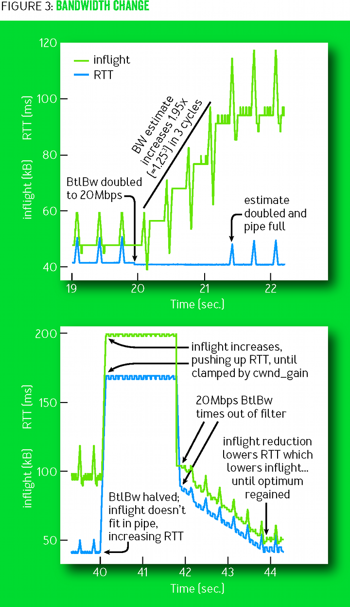


Figure 3

(Essentially, BBR is a simple example of a max-plus control system, a new approach to control systems based on nonstandard max-plus algebra [12]. This approach allows you to adapt the speed [controlled by the max transfer ratio] regardless of the queue growth [ controlled by the transfer coefficient average ]. Applied to our task, this comes down to a simple, unconditional control loop, where adaptation to changes in physical constraints is automatically carried out by changing the filters expressing these constraints. the topic would require the creation of multiple control loops combined into a complex state machine to achieve such a result).

Behavior when starting a single BBR stream

Modern implementations process events like startup (startup), shutdown (shutdown) and loss recovery (loss recovery) using algorithms that respond to "events" with a large number of lines of code. BBR uses the code above (in the previous chapter, “Matching Packet Flow with Delivery Path”) for everything. Event processing occurs by passing through a sequence of "states". The “states” themselves are defined by a table with one or several fixed values ​​of coefficients and exit criteria. Most of the time is spent in the ProbeBW state, which is described in the chapter “Behavior in a steady state”. The Startup and Drain states are used when starting the connection (Figure 4). To handle the connection, where the bandwidth increases by 12 orders of magnitude, in the Startup state, a binary search algorithm is implemented for BtlBw, where the transmission coefficient is used $$$2 / ln2$ for a twofold increase in transmission speed when delivery speed increases. So determined by BtlBw in $$$log_2BDP$ RTT, but at the same time creates an extra queue to $$$2BDP$ . As soon as Startup finds BtlBw, the BBR system enters the Drain state, which uses inverse Startup transfer coefficients to get rid of the excess queue, and then the ProbeBW state as soon as the inflight drops to the BDP line.


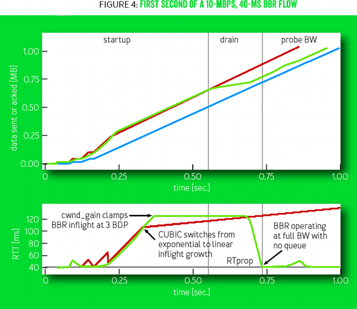
Figure 4

Figure 4 shows the first second of a 10-megabit BBR stream of 40 milliseconds. The top chart shows the time and sequence of events, as well as the progress of the sender (green) and recipient (blue): the amount of data transmitted and received. The red line shows the sender’s CUBIC performance under the same conditions. Vertical gray lines indicate moments of transition between BBR states. In the lower graph - the change in time of double pass packets (RTT) of both compounds. Please note that the time scale for this schedule corresponds to the time of receipt of confirmation of arrival (ack). Therefore, it may seem that the graphs seem to be shifted in time, but in fact the events below correspond to those moments when the BBR system finds out about these events and reacts.

The lower graph in Figure 4 compares BBR and CUBIC. At first, their behavior is almost the same, but BBR completely depletes the queue formed at the start of the connection, but CUBIC cannot do this. It does not have a trace model that would tell you how much of the data sent is redundant. Therefore, CUBIC less aggressively increases data transfer without confirming delivery, but this growth continues until the bottleneck buffer overflows and starts to drop packets, or until the receiver reaches the limit on the sent data without confirmation (TCP receive window).

Figure 5 shows the behavior of the RTT in the first eight seconds of the connection shown in the previous figure 4. The CUBIC technology (red) fills the entire available buffer, then spins between 70% and 100% of the fill every few seconds. After starting the connection, BBR (green) works almost without creating a queue.


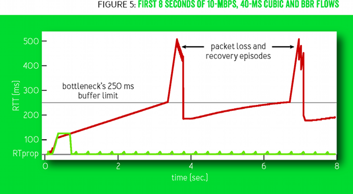
Figure 5

Behavior when multiple BBR streams meet in narrow place

Figure 6 shows how the bandwidth of several BBR streams converges in a fair channel partition with a 100 megabit / 10 millisecond bottleneck. Downward looking triangular structures are the states of the ProbeRTT connections in which self-synchronization speeds up the final convergence.


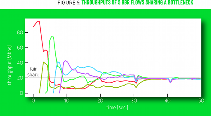
Figure 6

The cycles of change of the ProbeBW gain factors (Figure 2) stimulate larger flows to give way to smaller flows, as a result of which each flow understands its honest state. This happens quite quickly (several ProbeBW cycles), although injustice may persist if the threads that are late to the beginning of the redistribution overestimate RTprop due to the fact that previously started threads (temporarily) create a queue.

To find out the real RTProp, the stream moves to the left of the BDP line using the ProbeRTT state: if the RTProp score is not updated (that is, by measuring a smaller RTT) for many seconds, then BBR enters the ProbeRTT state, reducing the amount of data sent (inflight) to four packets for at least one double pass, and then returns to the previous state. When large flows enter the ProbeRTT state, many packets are removed from the queue, so several threads see the new value of RTprop (the new minimum RTT). Because of this, their RTprop scores are zeroed at the same time, so that they collectively enter the ProbeRTT state — and the queue shrinks even more, resulting in even more flows seeing the new value of RTprop, and so on. Such distributed coordination is a key factor at the same time for fair strip distribution and stability.

BBR synchronizes streams around the desired event, which is an empty queue in a narrow place. In contrast to this approach, regulating congestion on packet loss synchronizes flows around unwanted events, such as periodic queue growth and buffer overflow, which increases latency and packet loss.

Experience implementing B4 WAN to Google

Google's B4 network is a high-speed WAN network (wide-area network), built on conventional low-cost switches [15]. Losses on these switches with small buffers are mainly due to the random influx of small traffic bursts. In 2015, Google began to transfer working traffic from CUBIC to BBR. There were no problems or regressions, and since 2016, all B4 TCP traffic uses BBR. Figure 7 illustrates one reason for which this was done: the BBR capacity is consistently 2-25 times higher than that of CUBIC. We saw an even greater improvement, but found that 75% of BBR connections are limited to the TCP receive buffer in the core, which the network operations staff deliberately set to a low value (8 MB) to prevent CUBIC from flooding the network with megabytes of excess traffic without confirming delivery (if divide 8 MB to 200 ms of intercontinental RTT, then it will be 335 Mbit / s maximum). A manual increase in the receive buffer on a single US-Europe route instantly increased the BBR data transfer rate to 2 Gbit / s, while CUBIC remained at 15 Mbit / s — a 133-fold relative increase in throughput was predicted by Mathis and his colleagues in scientific the work of 1997. [17]


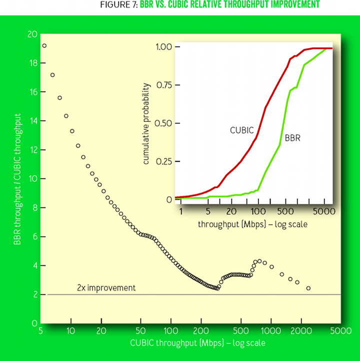
Figure 7

Figure 7 shows the relative improvement in BBR compared with CUBIC; on the sidebar - integral distribution functions (cumulative distribution functions, CDF) for bandwidth. The measurements were made using the active sensing service, which opens BBR and CUBIC permanent connections to remote data centers, then sends 8 MB of data every minute. The probes explore many B4 routes between North America, Europe and Asia.

A huge improvement is a direct consequence of the fact that BBR does not use packet loss as an indicator of congestion. To achieve full throughput for existing packet loss control methods, the loss level should be less than the inverse square of the BDP [17] (for example, less than one loss per 30 million packets for a 10 Gbit / s connection and 100 ms). Figure 8 compares the measured throughput at various levels of packet loss. In the CUBIC algorithm, the packet loss allowance is a structural property of the algorithm, and in BBR it is a configuration parameter. As the loss rate in BBR approaches the maximum Gain ProbeBW, the probability of measuring the delivery rate of a real BtlBw drops sharply, which leads to an underestimation from the max filter.


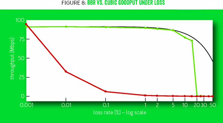
Figure 8

Figure 8 compares the useful bandwidth of the BBR and CUBIC in a 60-second stream at 100 Mb / s and 100 ms with a random loss of 0.001% to 50%. The capacity of CUBIC decreases 10 times at a loss of 0.1% and completely stalls at more than 1%. The maximum bandwidth is the share of the band minus packet losses ( $$$= 1 - lossRate$ ). BBR keeps at this level up to the level of losses of 5% and close to it up to 15%.

YouTube Edge Implementation Experience

BBR is deployed on YouTube and Google.com video servers. Google is conducting a small experiment in which a small percentage of users are randomly transferred to BBR or CUBIC. The BBR video playback shows a significant improvement in all user ratings of the service quality. Perhaps because the BBR behavior is more consistent and predictable. BBR only slightly improves connection bandwidth, because YouTube already adapts streaming speeds to levels far below BtlBw to minimize unnecessary network buffering and re-buffering. But even here, BBR reduces the average median RTT by 53% globally and more than 80% in developing countries.

Figure 9 shows the median improvement in RTT versus BBR and CUBIC statistics, with over 200 million YouTube video views measured on five continents during the week. More than half of all 7 billion mobile connections in the world connect at 2.5G at speeds from 8 to 114 Kbps [5], experiencing well-documented problems due to the fact that packet loss congestion control methods tend to overflow buffers [3]. The bottleneck in these systems is usually between the SGSN (the serving GPRS support node) [18] and the mobile device. The SGSN software runs on a standard PC platform with plenty of RAM, which often has megabytes of buffer between the Internet and a mobile device. Figure 10 compares the (emulated) SGSN delay between the Internet and the mobile device for BBR and CUBIC. Horizontal lines mark one of the most serious consequences: TCP adapts to long RTT delays, with the exception of a SYN packet initiating a connection that has a fixed timeout, depending on the operating system. When a mobile device receives a large data array (for example, from automatic software updates) via a large buffer SGSN, the device cannot establish any connection on the Internet until the queue is free (the confirming SYN ACK packet is delayed longer than the fixed SYN timeout) .


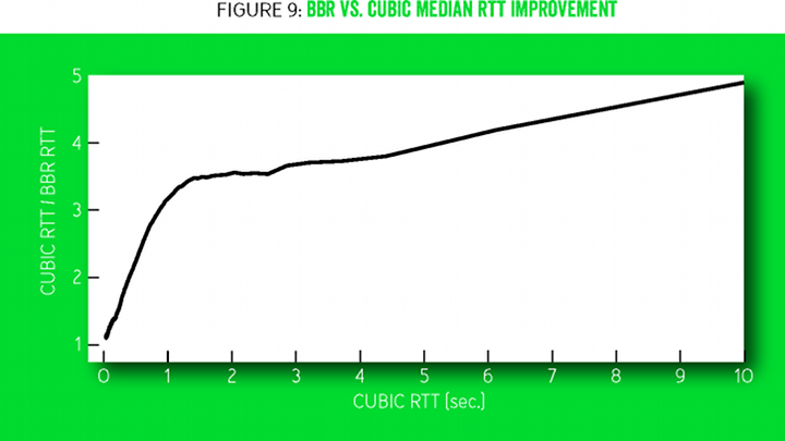
Figure 9

Figure 10 shows the median RTT changes in the steady state of the connection and the dependence on the buffer size on the 128 Kbps connection and 40 ms with eight BBR (green) or CUBIC (red) streams. BBR keeps the queue at the minimum values, regardless of the size of the bottleneck buffer and the number of active threads. CUBIC streams always fill the buffer, so the delay increases linearly with the buffer size.


Figure 10

Adaptive band in mobile cellular

Cellular systems adapt the bandwidth for each user partly depending on the forecast of requests, which takes into account the queue of packets destined for that user. Early versions of BBR were set up to create very small lines, which caused the connections to stop at low speeds. An increase in the peak value of pacing_gain for ProbeBW and an increase in queues resulted in a decrease in the stalled connections. This shows the possibility of excellent adaptation for some networks. With the current peak gain value $$$1.25 × BtlBw$ there is no degradation in any network compared to CUBIC.

Delayed and Stretched Packages ack

Cellular networks, WiFi and broadband networks often delay and accumulate ack packets [1]. When inflight is limited to one BDP, this leads to disruptions that reduce throughput. Increasing the cwnd_gain ProbeBW factor to two allowed us to continue smooth transmission at the predicted delivery speed, even when ack packets were delayed to a value of one RTT. This largely prevents breakdowns.

Current Bucket Limiters

The initial deployment of BBR on YouTube has shown that most of the Internet service providers in the world distort traffic using speed limits using the current bucket algorithm [7]. The bucket is usually full at the beginning of the connection, so BBR recognizes the BtlBw parameter for the underlying network. But as soon as the bucket is empty, all packets sent faster than (much smaller than BtlBw) bucket filling speed are discarded.BBR eventually recognizes this new delivery speed, but a cyclic change in ProbeBW gain leads to permanent moderate losses. To minimize the loss of the upstream bandwidth and the increase in application delays from these losses, we added a special limiter detector and an explicit limiter model in BBR. We are also actively exploring the best ways to eliminate the damage from speed limiters.

Competition with packet loss control methods

BBR comes down to honestly sharing the bottleneck bandwidth, whether in competition with other BBR streams or with streams managed by congestion loss control methods. Even when the latter fill the available buffer, ProbeBW still reliably shifts the BtlBw estimate towards fair flow separation, and ProbeRTT considers the RTProp score high enough for an eye for an eye to fair separation. However, unmanaged router buffers exceeding certain BDPs force outdated competitors with congestion control over packet loss to inflate the queue and grab more than is fair to them. Eliminating this is another area of ​​active research.

Conclusion

Rethinking traffic congestion management is a huge benefit. Instead of using events such as losses or buffer occupancy that only weakly correlate with congestion, BBR starts with the formal Kleinrock congestion model and its associated optimum operating point. The annoying conclusion about the “impossibility” of simultaneously determining critical delay and bandwidth parameters is bypassed by observing that they can be predicted simultaneously. Then, recent advances in control systems and estimation theory are applied to create a simple distributed control loop that approaches the optimum, fully utilizing the network while maintaining a small queue. The Google BBR implementation is available in the open source Linux kernel and is described in detail in the appendix to this article.

BBR technology is used on the Google B4 backbone, improving the throughput by orders of magnitude compared to CUBIC. It also takes place on Google and YouTube web servers, greatly reducing latency on all five continents tested to date, and especially in developing countries. BBR technology works exclusively on the sender's side and does not require changes in the protocol, on the recipient or on the network, which allows you to deploy it gradually. It depends only on RTT and packet delivery notifications, so it can be used in most Internet transport protocols.

Authors can be reached at bbr-dev@googlegroups.com.

Acknowledgments

The authors are grateful to Lena Kleinrock for pointing out how to properly regulate congestion. We are indebted to Larry Brakmo for his pioneering work on Vegas [2] and New Vegas congestion control systems, which anticipated many of the elements of BBR, as well as his advice and guidance at the initial stage of the development of BBR. We would also like to thank Eric Dumazet, Nandita Dukkipati, Jan Iyengar, Ian Swett, M. Fitz Nowlan, David Wetherall, Leon Wetherall, Leon, Leon Wetherall, Leon Wetherall, Leon Fitz Nowlan, David Wetherall, Leon Wetherall. Kontothanassis (Leonidas Kontothanassis), Amina Vahdat (Amin Vahdat) and the Google BwE development team and YouTube infrastructure for their invaluable help and support.

Appendix - a detailed description

The state machine for serial sensing

Gain pacing_gain controls how fast packets are sent relative to BtlBw, and this is the key to the intelligent BBR function. When pacing_gain is greater than one, the inflight increases and the gap between arrivals of packets decreases, which moves the connection to the right side in Figure 1. When pacing_gain is less than one, the opposite effect occurs, the connection moves to the left.

BBR uses pacing_gain to implement a simple sequential state sensing machine, which alternates between testing for a larger band and testing for a shorter time to double pass a packet. (It is not necessary to test for a smaller band because it is processed automatically by the BtlBw msx filter: new measurements reflect a drop, so BtlBw will correct itself as soon as the last old changes are removed from the filter by timeout. The RTprop min filter handles the increase in the delivery path in the same way) .

If the capacity of the bottleneck increases, BBR should send data faster to detect it. Similarly, if the real time of a double pass of a packet changes, it changes the BDP, and therefore the BDP must send data slower to keep the inflight below the BDP to measure the new RTprop. Therefore, the only way to detect these changes is to run experiments, sending faster to check for BtlBw magnification or sending more slowly to check for RTprop reduction. The frequency, scale, duration, and structure of these experiments differ depending on what is already known (starting the connection or the stable state) and on the behavior of the application that sends the data (intermittent or constant).

Steady state

BBRs spend most of their time in the ProbeBW state, probing a band using a method called gain cycling , which helps BBRs achieve high throughput, low queue lag, and convergence in an honest band section. Using gain cycling , BBR cyclically tries a series of values ​​for the pacing_gain gain . Eight cycle phases are used with the following values: 5/4, 3/4, 1, 1, 1, 1, 1, 1. Each phase usually goes through a predicted RTprop. This design allows the coefficient cycle to first probe the channel for more bandwidth with a pacing_gain value greater than 1.0, and then disperse any resulting queue using pacing_gainby the same amount less than 1.0, and then move at cruising speed with a short queue of coefficients exactly 1.0. The average gain for all phases is 1.0, because ProbeBW tends to average to equalize with the available bandwidth and, consequently, to maintain a high degree of band usage without increasing the queue. Notice that while the change cycles of the coefficient change the pacing_gain , the value of cwnd_gain invariably remains two, since delayed and extended acknowledgment packets may appear at any time (see the chapter on delayed and extended packets ack).

Moreover, to improve flow mixing and fair band separation, and to reduce queues when multiple BBR streams share a bottleneck, BBR randomly changes the phases of the ProbeBW cycle, randomly selecting the first phase among all values ​​except 3/4. Why doesn't the cycle start with 3/4? The main task of this coefficient value is to disperse any queue that may form during the application of the 5/4 factor, when the channel is already full. When a process exits the Drain or ProbeRTT state and enters ProbeBW, there is no queue, so the 3/4 factor does not perform its task. Using 3/4 in this context has only a negative effect: filling the channel in this phase will be 3/4, not 1. Thus, the beginning of the cycle with 3/4 has only a negative effect, but has no positive,and since the input to the ProbeBW state occurs at the start of any connection for a long time, BBR uses this small optimization.

BBRs work together to periodically empty a queue in a narrow place using a state called ProbeRTT. In any state other than ProbeRTT itself, if the RTProp score was not updated (for example, by measuring a smaller RTT) for more than 10 seconds, then BBR enters the ProbeRTT state and reduces cwnd to a very small value (four packets). Keeping such a minimum number of packets “in flight” for at least 200 ms and during one time of a double pass of a packet, BBR exits ProbeRTT and enters either Startup or ProbeBW, depending on the estimate whether the channel is already full.

BBR is designed to work most of the time (about 98%) in the ProbeBW state, and the rest of the time in ProbeRTT, based on a set of compromises. The ProbeRTT state lasts long enough (at least 200 ms) to allow threads with different RTT to have parallel ProbeRTT states, but at the same time it lasts a fairly short period of time to limit performance degradation to about two percent (200 ms / 10 seconds ). The RTprop filter window (10 seconds) is small enough to quickly adjust to changing traffic levels or changing routes, but large enough for interactive applications. Such applications (for example, web pages, remote procedure calls, video fragments) often demonstrate natural periods of silence or low activity in the windows of this window,where the flow rate is low enough or long enough to disperse the queue in a narrow place. Then the RTprop filter opportunistically matches these RTprop measurements, and the RTProp is updated without having to use ProbeRTT. Thus, threads typically only need to donate 2% of the band if multiple streams fill the channel abundantly throughout the whole RTProp window.

Startup Behavior

When a BBR stream starts, it performs its first (and fastest) sequential probe / empty queue process. Network bandwidth varies in the range of 10 ¹² - from a few bits to 100 gigabits per second. To find out the value of BtlBw with such a huge range change, BBR performs a binary search in velocity space. He very quickly finds BtlBw ($$l o g 2 B D P double passes of packets), but at the expense of creating a 2BDP queue at the last stage of the search. The search is performed in the Startup state in BBR, and the emptying of the created queue is in the Drain state.First, Startup exponentially increases the speed of sending data, doubling it at each round. To achieve such a fast sensing in the quietest way, when running, the values ​​of the gainfactors pacing_gainandcwnd_gain areset to$log_2BDP$

$$2 / l n 2 , to a minimum value that doubles the speed at which data is sent each round. Once the channel is filled, thecwnd_gaincoefficientlimits the queue size to$2/ln2$$$$(cwnd_gain - 1) × BDP$ .

In the start-up state, BBR assesses whether the channel is full by searching for a plateau in the BtlBw rating. If it turns out that several (three) rounds have passed, where attempts to double the delivery speed do not really give a big increase in speed (less than 25%), then he believes that he has reached BtlBw, so that he leaves the Startup state and enters the Drain state. BBR waits for three rounds to get convincing evidence that the delivery rate plateau observed by the sender is not a temporary effect influenced by the receiving window. Waiting for three rounds gives enough time for automatic tuning on the recipient's side to open the receiving window and for the BBR sender to detect the need to increase BtlBw: in the first round, the algorithm for automatically setting the receiving window increases the receiving window;in the second round, the sender fills the enlarged reception window; in the third round, the sender receives samples at an increased rate of delivery. Such a limit of three rounds proved itself as a result of implementation on YouTube.

In the Drain state, the BBR algorithm seeks to quickly empty the queue that was formed in the connection start state by switching to pacing_gain mode with inverse values ​​than those used in the Startup state. When the number of packets in flight corresponds to the BDP estimate, this means that BBR rates the queue as completely empty, but the channel is still full. Then the BBR exits the Drain state and enters ProbeBW.

Notice that the launch of the BBR connection and the slow start of the CUBIC both study the throughput of the bottleneck exponentially, doubling the dispatch rate in each round. However, they are radically different. First, BBR more reliably determines the available bandwidth because it does not stop searching in case of packet loss or (like CUBIC Hystart [10]) increasing the delay. Secondly, BBR smoothly increases the sending speed, while at CUBIC on each round (even with pacing) there is a surge in packets, and then a period of silence. Figure 4 shows the number of packets in flight and the observed RTT time for each acknowledgment message from BBR and CUBIC.

Transitional Response

The network path and the passage of traffic through it can experience sudden dramatic changes. In order to smoothly and reliably adapt to them, as well as reduce packet loss in these situations, BBR uses a number of strategies to implement its basic model. First, the BBR regards$$c w n d g a i n × B D P as a target, to which the currentcwndcarefully approaches from the bottom, increasingcwndeach time by no more than the amount of data for which delivery confirmations have arrived. Second, with a retransmission timeout, which means that the sender considers all packets lost in flight, BBR conservatively lowerscwnd$cwnd_gain×BDP$up to one packet and sends a single packet (just like congestion algorithms for packet loss, such as CUBIC). In the end, when the sender notices a packet loss, but there are still packets in flight, in the first stage of the loss recovery process, BBR temporarily reduces the sending speed to the level of the current delivery speed; on the second and subsequent loss recovery rounds, he checks that the sending speed never exceeds the current delivery speed more than twice. This significantly reduces losses in transient situations when BBR collides with speed limiters or competes with other streams in a buffer comparable to the size of a BDP.

Links

1. Abrahamsson, M. 2015. TCP ACK suppression. IETF AQM mailing list; https://www.ietf.org/mail-archive/web/aqm/current/msg01480.html .

2. Brakmo, LS, Peterson, LL 1995. TCP Vegas: end-to-end congestion avoidance on a global Internet. IEEE Journal on Selected Areas in Communications 13 (8): 1465-1480.

3. Chakravorty, R., Cartwright, J., Pratt, I. 2002. Practical experience with TCP over GPRS. In IEEE GLOBECOM.

4. Corbet, J. 2013. TSO sizing and the FQ scheduler. LWN.net; https://lwn.net/Articles/564978/ .

5. Ericsson. 2015 Ericsson Mobility Report (June); https://www.ericsson.com/res/docs/2015/ericsson-mobility-report-june-2015.pdf .

6. ESnet. Application tuning to optimize international astronomy workflow from NERSC to LFI-DPC at INAF-OATs; http://fasterdata.es.net/data-transfer-tools/case-studies/nersc-astronomy/ .

7. Flach, T., Papageorge, P., Terzis, A., Pedrosa, L., Cheng, Y., Karim, T., Katz-Bassett, E., Govindan, R. 2016. An Internet-wide analysis of traffic policing. ACM SIGCOMM: 468-482.

8. Gail, R., Kleinrock, L. 1981. An invariant property of computer network power. Conference Record, International Conference on Communications: 63.1.1-63.1.5.

9. Gettys, J., Nichols, K. 2011. Bufferbloat: dark buffers in the Internet. acmqueue 9 (11); http://queue.acm.org/detail.cfm?id=2071893 .

10. Ha, S., Rhee, I. 2011. Taming the elephants: new TCP slow start. Computer Networks 55 (9): 2092-2110.

11. Ha, S., Rhee, I., Xu, L. 2008. CUBIC: a new TCP-friendly high-speed TCP variant. ACM SIGOPS Operating Systems Review 42 (5): 64-74.

12. Heidergott, B., Olsder, GJ, Van Der Woude, J. 2014. Max. Algebra and its Applications. Princeton University Press.

13. Jacobson, V. 1988. Congestion avoidance and control. ACM SIGCOMM Computer Communication Review 18 (4): 314-329.

14. Jaffe, J. 1981. Flow control power is nondecentralizable. IEEE Transactions on Communications 29 (9): 1301-1306.

15. Jain, S., Kumar, A., Mandal, S., Ong, J., Poutievski, L., Singh, A., Venkata, S., Wanderer, J., Zhou, J., Zhu, M ., et al. 2013. B4: experience with a globally-deployed software defined WAN. ACM SIGCOMM Computer Communication Review 43 (4): 3-14.

16. Kleinrock, L. 1979. Power and deterministic rules of thumb for computer communications. In Conference Record, International Conference on Communications: 43.1.1-43.1.10.

17. Mathis, M., Semke, J., Mahdavi, J., Ott, T. 1997. The congestion avoidance algorithm. ACM SIGCOMM Computer Communication Review 27 (3): 67-82.

18. Wikipedia. Serving GPRS support node in the GPRS core network; https://en.wikipedia.org/wiki/GPRS_core_network#Serving_GPRS_support_node_.28SGSN.29 .


« »
Aiman Erbad, Charles «Buck» Krasic

« »
Kevin Fall, Steve McCanne

« - »
Dennis Abts, Bob Felderman

— Google make-tcp-fast, — . TFO (TCP Fast Open), TLP (Tail Loss Probe), RACK, fq/pacing git TCP Linux .