Interesting clustering algorithms, part two: DBSCAN
Part One - Affinity Propagation
Part Two - DBSCAN
Part Three - Time Series Clustering
Part Four - Self-Organizing Maps (SOM)
Part Five - Growing Neural Gas (GNG)
We will go deep into a little more untamed jungle of Data Science. Today in line for preparation of the clustering algorithm DBSCAN. I ask people who have encountered or are going to encounter data clustering, in which there are clots of arbitrary shape, under the cut - today your arsenal will be replenished with an excellent tool.
DBSCAN (Density-based spatial clustering of applications with noise, the density algorithm of spatial clustering with the presence of noise), as the name implies, operates on data density. At the entrance, he asks for a familiar proximity matrix and two mysterious parameters - the radius - neighborhood and number of neighbors. So at once you will not understand how to select them, and here is the density, and why DBSCAN deals well with noisy data. Without this, it is difficult to determine the limits of its applicability.
')
Let's figure it out. As in the previous article , I propose to first turn to the speculative description of the algorithm, and then bring mathematics under it. I like the explanation that I stumbled upon Quora , so I will not reinvent the wheel, and will reproduce it here with some minor modifications.
In a giant hall a crowd of people celebrates someone's birthday. Someone loiter alone, but most - with friends. Some companies are simply crowded with a crowd, some - dance in circles or dance lambadas.
We want to divide the people in the hall into groups.
But how to select groups of such different forms, but still not forget about the loners? Let's try to estimate the density of the crowd around each person. Probably, if the crowd density between two people is above a certain threshold, then they belong to the same company. In fact, it will be strange if the people driving the train will belong to different groups, even if the density of the chain between them varies within certain limits.
We will say that a crowd has gathered next to a certain person if several other people are standing close to him. Yeah, it is immediately clear that you need to set two parameters. What does “close” mean? Take some intuitive distance. Let's say if people can touch each other's heads, then they are close. About a meter. Now, how many "several other people"? Suppose three people. Two can walk and just like that, but the third is definitely superfluous.
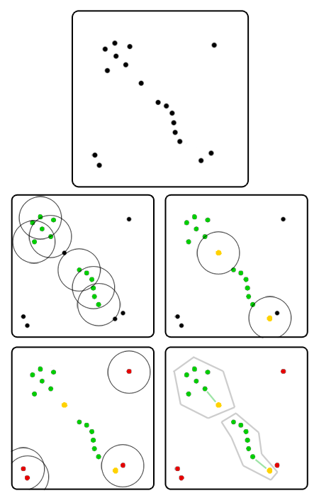
Let everyone calculate how many people are in a radius of a meter from him. All who have at least three neighbors, take up the green flags. Now they are fundamental elements, they form groups.
Let us turn to people who have less than three neighbors. Select those with at least one neighbor holding a green flag and hand them yellow flags. We say that they are on the border of groups.
There are loners who have not only three no neighbors, so neither of them holds the green flag. Give them red flags. We assume that they do not belong to any group.
Thus, if from one person to another you can create a chain of “green” people, then these two people belong to the same group. It is obvious that all such clusters are divided either by empty space or by people with yellow flags. They can be numbered: each in group No. 1 can reach along the chain of hands of each other in group No. 1, but nobody in No. 2, No. 3, and so on. Same for other groups.
If there is only one “green” neighbor next to a person with a yellow flag, he will belong to the group to which his neighbor belongs. If there are several such neighbors, and they have different groups, then you have to choose. Here you can use different methods - see who is the nearest neighbor, for example. We'll have to somehow bypass the boundary cases, but that's okay.
As a rule, it makes no sense to tag all the indigenous elements of the crowd at once. Since from each root element of the group you can hold a chain to each other, it’s all the same from which one to start the detour - sooner or later you will find everyone. An iterative version is better suited here:
We introduce several definitions. Let some symmetric distance function be given and constants and . Then
Choose some root object from the dataset, mark it and put all of its directly densely accessible neighbors in the bypass list. Now for each from the list: mark this point, and if it is also a root, add all of its neighbors to the traversal list. It is trivially proved that clusters of labeled points formed in the course of this algorithm are maximal (i.e., they cannot be extended with one more point so that the conditions are satisfied) and are connected in the sense of dense reachability. It follows that if we did not go around all the points, you can restart the crawl from some other root object, and the new cluster will not absorb the previous one.
Wait a second ... Yes, it's a disguised width traversal with restrictions! So it is, only added to the bells and whistles with the conditions of bypass and boundary points.
Wikipedia graciously provides the pseudocode framework for the algorithm.
Or, for those who do not like pseudocode, a very very naive implementation on python
An example of a more correct implementation of DBSCAN on python can be found in the sklearn package. The implementation example in Matlab was already on Habré . If you prefer R, take a look here and here .
Ideally, DBSCAN can achieve complexity , but do not really count on it. If not recalculate every time points, then the expected complexity - . Worst case (bad data or brute force implementation) - . DBSCAN naive implementations love to eat off memory for the distance matrix - this is clearly redundant. Many versions of the algorithm are able to work with more gentle data structures: sklearn and R implementations can be optimized using the KD-tree right out of the box. Unfortunately, because of bugs, this does not always work.
DBSCAN with a non-random edge point processing rule is deterministic. However, most implementations to speed up the work and reduce the number of parameters give edge points to the first clusters that reached them. For example, the central yellow point in the picture above in different launches may belong to both the lower and upper cluster. As a rule, this slightly affects the quality of the algorithm, because the cluster still does not spread further through the boundary points - a situation where the point jumps from cluster to cluster and “opens the way” to other points is impossible.
DBSCAN does not independently calculate cluster centers; however, this is hardly a problem, especially considering the arbitrary shape of clusters. But DBSCAN automatically detects outliers, which is pretty cool.
Ratio where - the dimension of space, can be intuitively considered as the threshold density of data points in the region of space. It is expected that with the same ratio , and the results will be about the same. Sometimes this is true, but there is a reason why the algorithm needs to specify two parameters, and not one. Firstly, the typical distance between points in different datasets is different - the radius must always be explicitly set. Secondly, they play the role of heterogeneity dataset. The more and , the more the algorithm tends to "forgive" density variations in clusters. On the one hand, this can be useful: it is unpleasant to see “holes” in a cluster, where there simply is not enough data. On the other hand, it is harmful when there is no clear boundary between clusters or noise creates a “bridge” between clusters. Then DBSCAN will easily connect two different groups. In the balance of these parameters lies the difficulty of using DBSCAN: real data sets contain clusters of different densities with borders of varying degrees of blurring. In conditions when the density of some borders between clusters is greater than or equal to the density of some separate clusters, one has to sacrifice something.
There are DBSCAN options that can mitigate this problem. The idea is to tweak in different areas in the course of the algorithm. Unfortunately, the number of algorithm parameters increases.
There are heuristics to choose from. and . Most often, this method and its variations are used:
To get a slightly better insight about and , you can play around with the parameters online here . Choose DBSCAN Rings and pull the sliders.
In any case, the main disadvantages of DBSCAN are the inability to connect clusters through openings, and, conversely, the ability to connect clearly different clusters through densely populated jumpers. Partly, therefore, when increasing the data dimension insidious stab in the back causes curse dimension: the more , the more places where openings or bridges can occur. I recall that an adequate number of data points increases exponentially with increasing .
DBSCAN is highly modifiable. Here it is suggested to cross DBSCAN with k-means for acceleration. The article demonstrates beautiful graphics, but I don’t quite understand how such an algorithm appears on clusters of dimensions much smaller than the dimension of space. See also the crossing variant with Gaussian Mixture and the non-parametric version of the algorithm.
DBSCAN is parallelized, but it is not trivial to do this effectively. If process number 1 found that many - subcluster, and process number 2, that - subcluster, and then and can be combined. The problem is to notice in time that the intersection of sets is not empty, because the constant synchronization of the lists greatly undermines performance. See these articles for implementation options.
Use DBSCAN when:
DBSCAN has a history of successful applications. For example, you can note its use in tasks:
At this point I would like to complete the second part of the cycle. I hope the article was useful to you, and now you know when DBSCAN should be tried in data analysis tasks, and when it should not be used.
Part Two - DBSCAN
Part Three - Time Series Clustering
Part Four - Self-Organizing Maps (SOM)
Part Five - Growing Neural Gas (GNG)
We will go deep into a little more untamed jungle of Data Science. Today in line for preparation of the clustering algorithm DBSCAN. I ask people who have encountered or are going to encounter data clustering, in which there are clots of arbitrary shape, under the cut - today your arsenal will be replenished with an excellent tool.
DBSCAN (Density-based spatial clustering of applications with noise, the density algorithm of spatial clustering with the presence of noise), as the name implies, operates on data density. At the entrance, he asks for a familiar proximity matrix and two mysterious parameters - the radius - neighborhood and number of neighbors. So at once you will not understand how to select them, and here is the density, and why DBSCAN deals well with noisy data. Without this, it is difficult to determine the limits of its applicability.
')
Let's figure it out. As in the previous article , I propose to first turn to the speculative description of the algorithm, and then bring mathematics under it. I like the explanation that I stumbled upon Quora , so I will not reinvent the wheel, and will reproduce it here with some minor modifications.
Intuitive explanation
In a giant hall a crowd of people celebrates someone's birthday. Someone loiter alone, but most - with friends. Some companies are simply crowded with a crowd, some - dance in circles or dance lambadas.
We want to divide the people in the hall into groups.
But how to select groups of such different forms, but still not forget about the loners? Let's try to estimate the density of the crowd around each person. Probably, if the crowd density between two people is above a certain threshold, then they belong to the same company. In fact, it will be strange if the people driving the train will belong to different groups, even if the density of the chain between them varies within certain limits.
We will say that a crowd has gathered next to a certain person if several other people are standing close to him. Yeah, it is immediately clear that you need to set two parameters. What does “close” mean? Take some intuitive distance. Let's say if people can touch each other's heads, then they are close. About a meter. Now, how many "several other people"? Suppose three people. Two can walk and just like that, but the third is definitely superfluous.
Let everyone calculate how many people are in a radius of a meter from him. All who have at least three neighbors, take up the green flags. Now they are fundamental elements, they form groups.
Let us turn to people who have less than three neighbors. Select those with at least one neighbor holding a green flag and hand them yellow flags. We say that they are on the border of groups.
There are loners who have not only three no neighbors, so neither of them holds the green flag. Give them red flags. We assume that they do not belong to any group.
Thus, if from one person to another you can create a chain of “green” people, then these two people belong to the same group. It is obvious that all such clusters are divided either by empty space or by people with yellow flags. They can be numbered: each in group No. 1 can reach along the chain of hands of each other in group No. 1, but nobody in No. 2, No. 3, and so on. Same for other groups.
If there is only one “green” neighbor next to a person with a yellow flag, he will belong to the group to which his neighbor belongs. If there are several such neighbors, and they have different groups, then you have to choose. Here you can use different methods - see who is the nearest neighbor, for example. We'll have to somehow bypass the boundary cases, but that's okay.
As a rule, it makes no sense to tag all the indigenous elements of the crowd at once. Since from each root element of the group you can hold a chain to each other, it’s all the same from which one to start the detour - sooner or later you will find everyone. An iterative version is better suited here:
- We approach a random person from the crowd.
- If there are fewer than three people next to him, transfer him to the list of possible hermits and choose someone else.
- Otherwise:
- Exclude it from the list of people who need to get around.
- We give this person a green flag and create a new group, in which he is currently the only inhabitant.
- We go around all its neighbors. If his neighbor is already on the list of potential singles or there are few other people next to him, then the edge of the crowd is in front of us. For simplicity, you can immediately mark it with a yellow flag, attach it to the group and continue the walk. If the neighbor also turns out to be “green”, then he does not start a new group, but joins the already created one; in addition, we add to the neighbor's neighbor traversal list. Repeat this item until the crawl list is empty.
- Repeat steps 1-3, until somehow we do not go around all the people.
- We deal with the list of hermits. If in step 3 we have already scattered all the edges, then only single emissions remain in it - you can immediately finish. If not, then you need to somehow distribute the people remaining in the list.
Formal approach
We introduce several definitions. Let some symmetric distance function be given and constants and . Then
- Let's call the region , for which , - neighborhood of the object .
- Root object or nuclear object degree called an object - whose neighborhood contains at least objects: .
- An object directly tight-reachable from the object , if a and - root object.
- An object tight-reachable from the object , if a such that directly tight-reachable from
Choose some root object from the dataset, mark it and put all of its directly densely accessible neighbors in the bypass list. Now for each from the list: mark this point, and if it is also a root, add all of its neighbors to the traversal list. It is trivially proved that clusters of labeled points formed in the course of this algorithm are maximal (i.e., they cannot be extended with one more point so that the conditions are satisfied) and are connected in the sense of dense reachability. It follows that if we did not go around all the points, you can restart the crawl from some other root object, and the new cluster will not absorb the previous one.
Wait a second ... Yes, it's a disguised width traversal with restrictions! So it is, only added to the bells and whistles with the conditions of bypass and boundary points.
Wikipedia graciously provides the pseudocode framework for the algorithm.
Pseudocode
DBSCAN(D, eps, MinPts) { C = 0 for each point P in dataset D { if P is visited continue next point mark P as visited NeighborPts = regionQuery(P, eps) if sizeof(NeighborPts) < MinPts mark P as NOISE else { C = next cluster expandCluster(P, NeighborPts, C, eps, MinPts) } } } expandCluster(P, NeighborPts, C, eps, MinPts) { add P to cluster C for each point Q in NeighborPts { if Q is not visited { mark Q as visited QNeighborPts = regionQuery(Q, eps) if sizeof(QNeighborPts) >= MinPts NeighborPts = NeighborPts joined with QNeighborPts } if Q is not yet member of any cluster add Q to cluster C } } regionQuery(P, eps) return all points within P eps-neighborhood (including P) Or, for those who do not like pseudocode, a very very naive implementation on python
Python
from itertools import cycle from math import hypot from numpy import random import matplotlib.pyplot as plt def dbscan_naive(P, eps, m, distance): NOISE = 0 C = 0 visited_points = set() clustered_points = set() clusters = {NOISE: []} def region_query(p): return [q for q in P if distance(p, q) < eps] def expand_cluster(p, neighbours): if C not in clusters: clusters[C] = [] clusters[C].append(p) clustered_points.add(p) while neighbours: q = neighbours.pop() if q not in visited_points: visited_points.add(q) neighbourz = region_query(q) if len(neighbourz) > m: neighbours.extend(neighbourz) if q not in clustered_points: clustered_points.add(q) clusters[C].append(q) if q in clusters[NOISE]: clusters[NOISE].remove(q) for p in P: if p in visited_points: continue visited_points.add(p) neighbours = region_query(p) if len(neighbours) < m: clusters[NOISE].append(p) else: C += 1 expand_cluster(p, neighbours) return clusters if __name__ == "__main__": P = [(random.randn()/6, random.randn()/6) for i in range(150)] P.extend([(random.randn()/4 + 2.5, random.randn()/5) for i in range(150)]) P.extend([(random.randn()/5 + 1, random.randn()/2 + 1) for i in range(150)]) P.extend([(i/25 - 1, + random.randn()/20 - 1) for i in range(100)]) P.extend([(i/25 - 2.5, 3 - (i/50 - 2)**2 + random.randn()/20) for i in range(150)]) clusters = dbscan_naive(P, 0.2, 4, lambda x, y: hypot(x[0] - y[0], x[1] - y[1])) for c, points in zip(cycle('bgrcmykgrcmykgrcmykgrcmykgrcmykgrcmyk'), clusters.values()): X = [p[0] for p in points] Y = [p[1] for p in points] plt.scatter(X, Y, c=c) plt.show() An example of a more correct implementation of DBSCAN on python can be found in the sklearn package. The implementation example in Matlab was already on Habré . If you prefer R, take a look here and here .
Nuances of application
Ideally, DBSCAN can achieve complexity , but do not really count on it. If not recalculate every time points, then the expected complexity - . Worst case (bad data or brute force implementation) - . DBSCAN naive implementations love to eat off memory for the distance matrix - this is clearly redundant. Many versions of the algorithm are able to work with more gentle data structures: sklearn and R implementations can be optimized using the KD-tree right out of the box. Unfortunately, because of bugs, this does not always work.
DBSCAN with a non-random edge point processing rule is deterministic. However, most implementations to speed up the work and reduce the number of parameters give edge points to the first clusters that reached them. For example, the central yellow point in the picture above in different launches may belong to both the lower and upper cluster. As a rule, this slightly affects the quality of the algorithm, because the cluster still does not spread further through the boundary points - a situation where the point jumps from cluster to cluster and “opens the way” to other points is impossible.
DBSCAN does not independently calculate cluster centers; however, this is hardly a problem, especially considering the arbitrary shape of clusters. But DBSCAN automatically detects outliers, which is pretty cool.
Ratio where - the dimension of space, can be intuitively considered as the threshold density of data points in the region of space. It is expected that with the same ratio , and the results will be about the same. Sometimes this is true, but there is a reason why the algorithm needs to specify two parameters, and not one. Firstly, the typical distance between points in different datasets is different - the radius must always be explicitly set. Secondly, they play the role of heterogeneity dataset. The more and , the more the algorithm tends to "forgive" density variations in clusters. On the one hand, this can be useful: it is unpleasant to see “holes” in a cluster, where there simply is not enough data. On the other hand, it is harmful when there is no clear boundary between clusters or noise creates a “bridge” between clusters. Then DBSCAN will easily connect two different groups. In the balance of these parameters lies the difficulty of using DBSCAN: real data sets contain clusters of different densities with borders of varying degrees of blurring. In conditions when the density of some borders between clusters is greater than or equal to the density of some separate clusters, one has to sacrifice something.
There are DBSCAN options that can mitigate this problem. The idea is to tweak in different areas in the course of the algorithm. Unfortunately, the number of algorithm parameters increases.
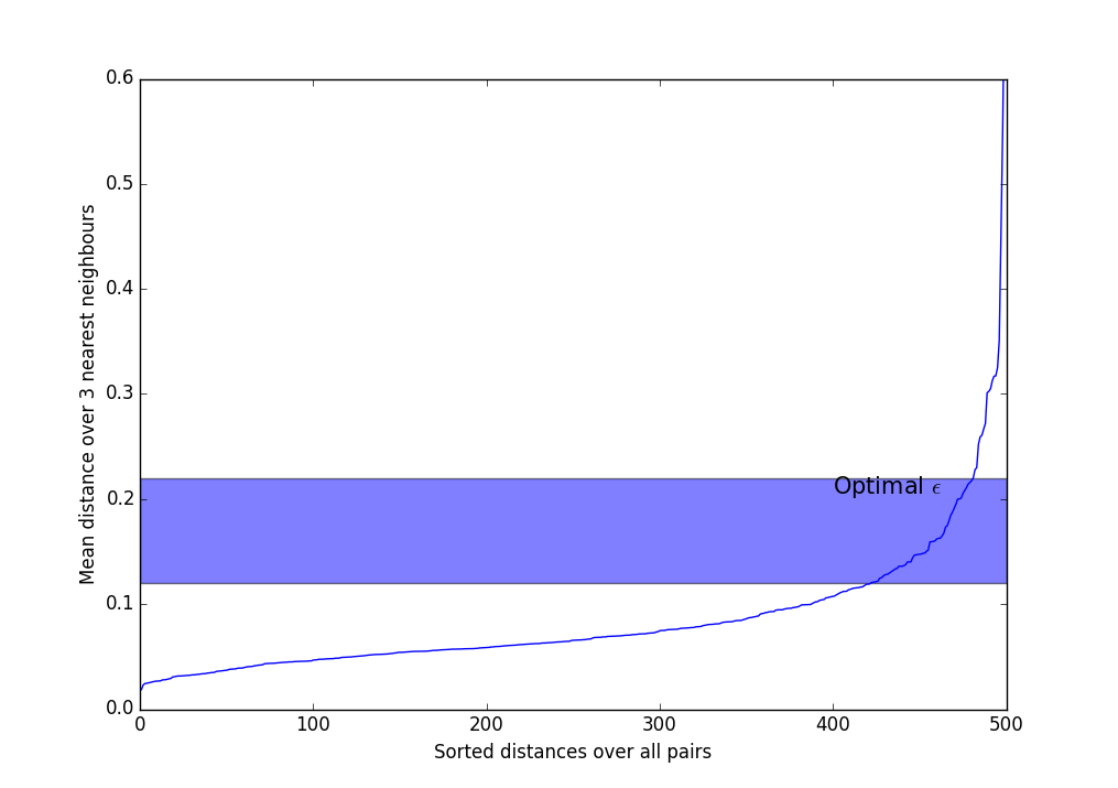
There are heuristics to choose from. and . Most often, this method and its variations are used:
- Select . Usually, values from 3 to 9 are used, the more non-uniform the data is expected to be, and the greater the noise level, the greater should be .
- Calculate the average distance over nearest neighbors for each point. Those. if a , you need to choose the three nearest neighbors, add the distances to them and divide by three.
- We sort the obtained values in ascending order and display them on the screen.
- We see something like such a sharply increasing graph. Should take somewhere in the band where the most extreme bend occurs. The more , the more clusters are obtained, and the less they will be.
To get a slightly better insight about and , you can play around with the parameters online here . Choose DBSCAN Rings and pull the sliders.
In any case, the main disadvantages of DBSCAN are the inability to connect clusters through openings, and, conversely, the ability to connect clearly different clusters through densely populated jumpers. Partly, therefore, when increasing the data dimension insidious stab in the back causes curse dimension: the more , the more places where openings or bridges can occur. I recall that an adequate number of data points increases exponentially with increasing .
DBSCAN is highly modifiable. Here it is suggested to cross DBSCAN with k-means for acceleration. The article demonstrates beautiful graphics, but I don’t quite understand how such an algorithm appears on clusters of dimensions much smaller than the dimension of space. See also the crossing variant with Gaussian Mixture and the non-parametric version of the algorithm.
DBSCAN is parallelized, but it is not trivial to do this effectively. If process number 1 found that many - subcluster, and process number 2, that - subcluster, and then and can be combined. The problem is to notice in time that the intersection of sets is not empty, because the constant synchronization of the lists greatly undermines performance. See these articles for implementation options.
Experiments
Don't open, pictures inside
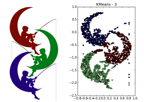
For splitting the same data using k-means and Affinity propagation, see my previous post .
DBSCAN works fine on dense clusters that are well separated from each other. Moreover, their form is completely irrelevant. Perhaps DBSCAN detects clusters of small dimensionality better than all unspecialized algorithms.


Please note that in the example with four straight lines, depending on the parameters, both 8 and 4 clusters can be obtained due to discontinuities in the straight lines. In general, this is often a desirable behavior — it is not known whether the distribution is true or if we simply lack data. Here we were lucky: the distance between the straight lines is larger than the size of the opening. Also note which points belong to different clusters in the spiral example. The length of the spiral, referred to the cluster, increases with decreasing number of neighbors, since Closer to the center of the helix, the points are closer.
Clusters of different sizes are determined well ...
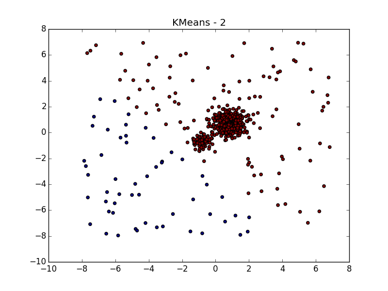
... even when the data is very noisy. Here, DBSCAN has an advantage over k-means, which will easily take asymmetrically distributed emissions per cluster.
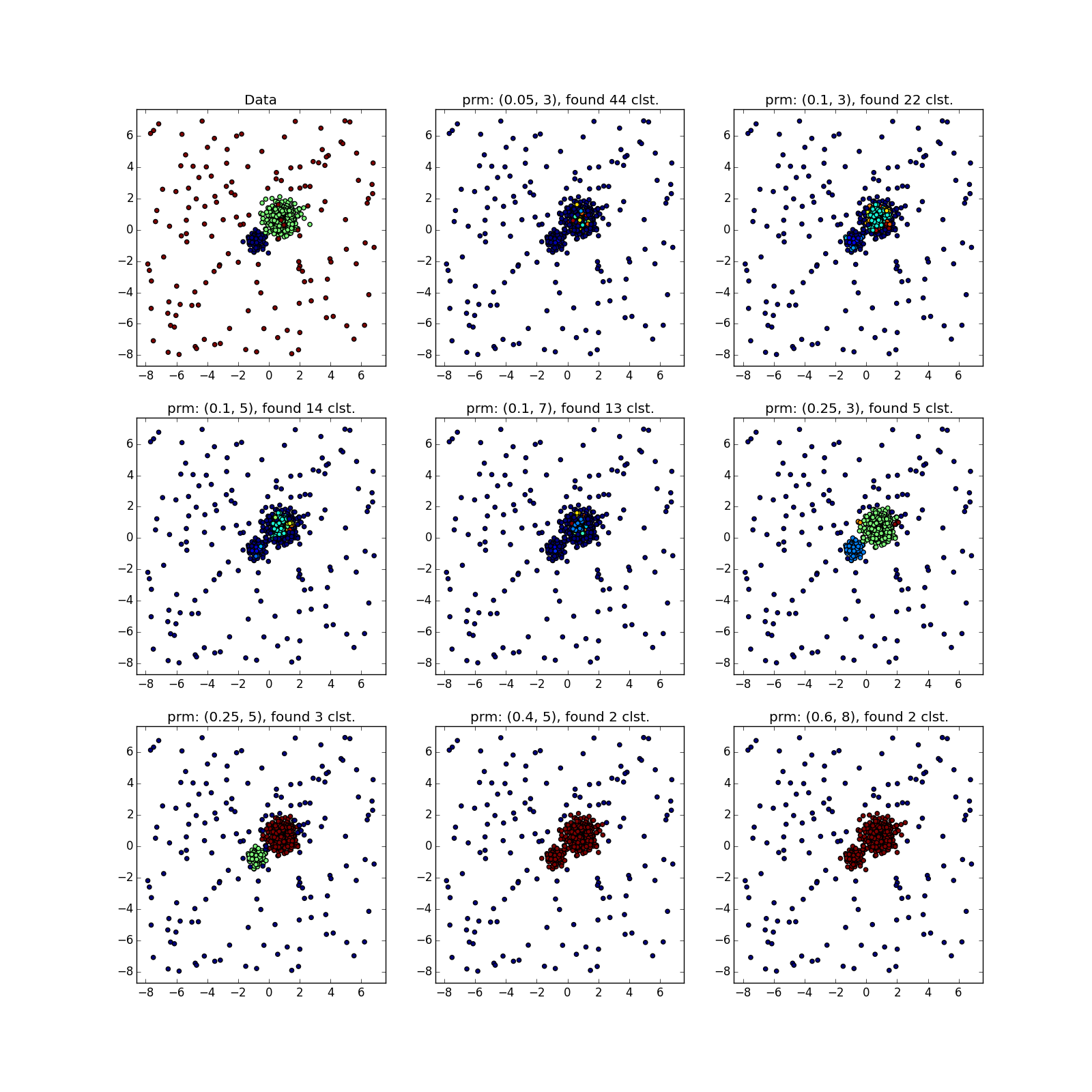
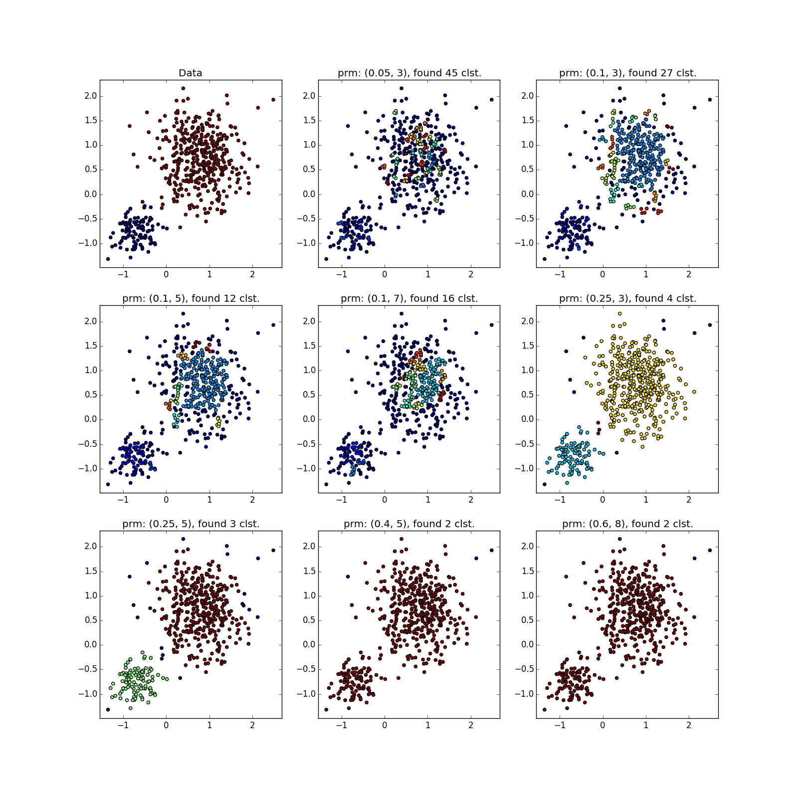
But with clusters of different densities, everything is not so rosy. DBSCAN either finds only a cluster of greater density, or the whole thing.
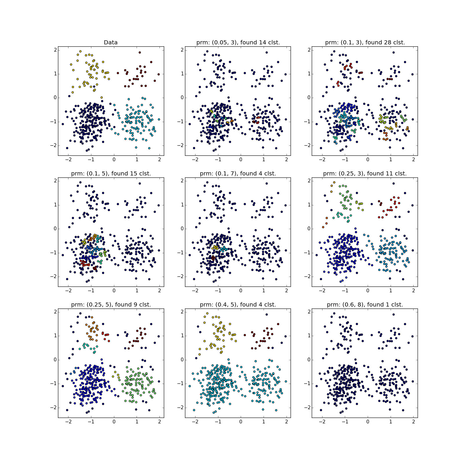
You can see something suspicious except by luck, or by chasing DBSCAN several times with different parameters. In fact - the manual execution of variations of the algorithm, about which I mentioned above.
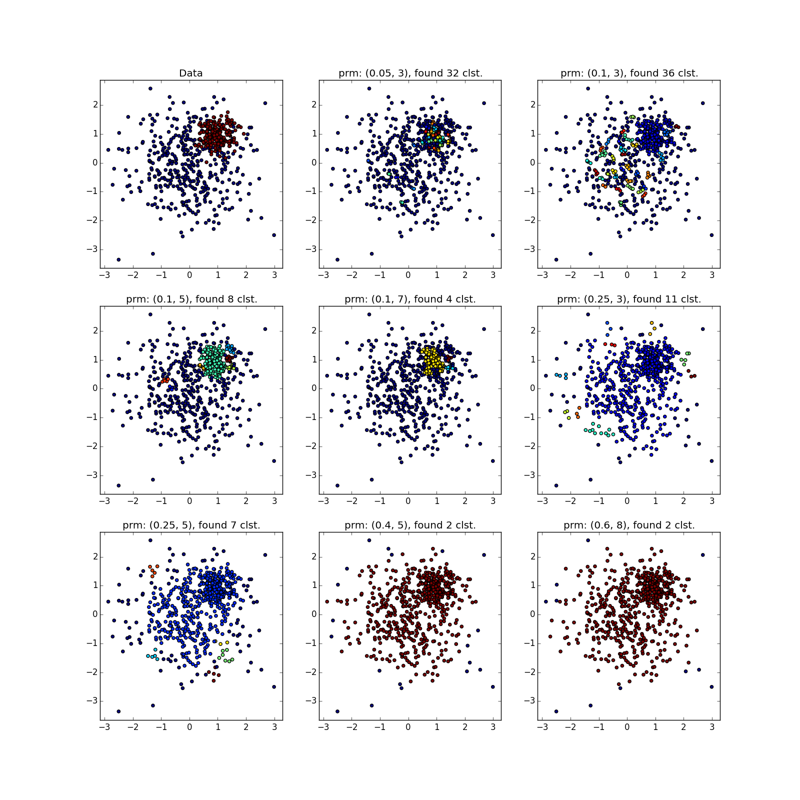
With more complex distributions - how lucky. If they are well separable, DBSCAN works. See (0.4, 5) - an excellent partition, although a bit too many points, which the algorithm considered outliers.

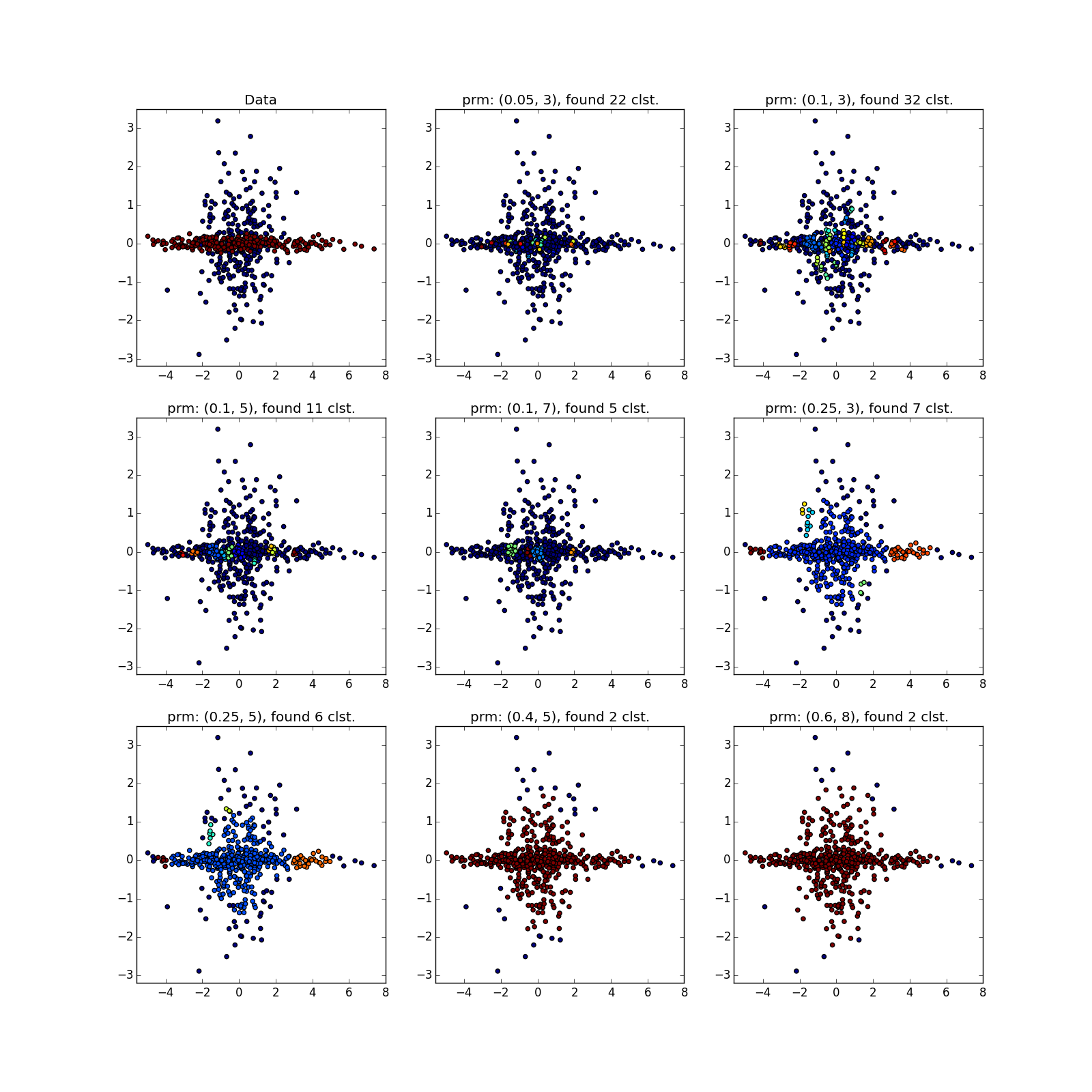
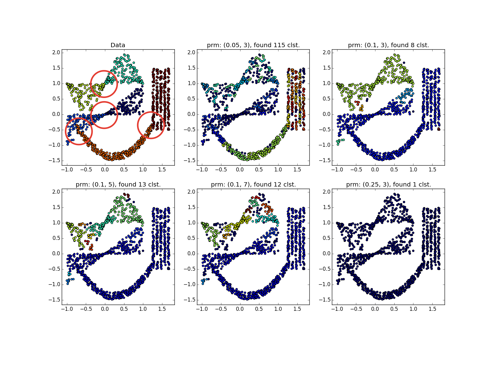
If jumpers prevail, not so much. Many points have accumulated in the selected places, because of which DBSCAN cannot distinguish between the “petals” of obviously different distributions.
DBSCAN works fine on dense clusters that are well separated from each other. Moreover, their form is completely irrelevant. Perhaps DBSCAN detects clusters of small dimensionality better than all unspecialized algorithms.
Please note that in the example with four straight lines, depending on the parameters, both 8 and 4 clusters can be obtained due to discontinuities in the straight lines. In general, this is often a desirable behavior — it is not known whether the distribution is true or if we simply lack data. Here we were lucky: the distance between the straight lines is larger than the size of the opening. Also note which points belong to different clusters in the spiral example. The length of the spiral, referred to the cluster, increases with decreasing number of neighbors, since Closer to the center of the helix, the points are closer.
Clusters of different sizes are determined well ...
... even when the data is very noisy. Here, DBSCAN has an advantage over k-means, which will easily take asymmetrically distributed emissions per cluster.
But with clusters of different densities, everything is not so rosy. DBSCAN either finds only a cluster of greater density, or the whole thing.
You can see something suspicious except by luck, or by chasing DBSCAN several times with different parameters. In fact - the manual execution of variations of the algorithm, about which I mentioned above.
With more complex distributions - how lucky. If they are well separable, DBSCAN works. See (0.4, 5) - an excellent partition, although a bit too many points, which the algorithm considered outliers.
If jumpers prevail, not so much. Many points have accumulated in the selected places, because of which DBSCAN cannot distinguish between the “petals” of obviously different distributions.
Total
Use DBSCAN when:
- You have a big measure ( ) dataset. Even If at hand an optimized and parallelized implementation.
- The function of proximity is known in advance, symmetric, preferably not very complex. KD-Tree optimization often works only with Euclidean distance.
- You expect to see clots of data of an exotic form: nested and anomalous clusters, folds of small dimension.
- The density of the boundaries between the bunches is less than the density of the least dense cluster. Better if the clusters are completely separated from each other.
- The complexity of the elements dataset does not matter. However, they should be enough so that there are no strong discontinuities in density (see the previous paragraph).
- The number of elements in a cluster can vary arbitrarily.
- The amount of emissions does not matter (within reasonable limits) if they are scattered over a large volume.
- The number of clusters does not matter.
DBSCAN has a history of successful applications. For example, you can note its use in tasks:
- Detection of social circles
- Image segmentation
- Modeling the behavior of website users
- Pre-processing in a weather prediction problem
At this point I would like to complete the second part of the cycle. I hope the article was useful to you, and now you know when DBSCAN should be tried in data analysis tasks, and when it should not be used.
Source: https://habr.com/ru/post/322034/
All Articles