We create a neural network InceptionV3 for image recognition

Hi, Habr! Under the cat we will talk about the implementation of the InceptionV3 convolutional neural network architecture using the Keras framework. I decided to write an article after getting acquainted with the tutorial " Building powerful classification models using a small amount of data ." With the approval of the author of the tutorial, I slightly changed the content of my article. Unlike the VGG16 neural network proposed by the author, we will train the Google deep neural network Inception V3 , which is already preinstalled in Keras.
You will learn:
')
- Import the Inception V3 neural network from the Keras library;
- Adjust the network: load weights, change the upper part of the model ( fc-layers ), thus fitting the model to the binary classification;
- To fine-tune the lower convolutional layer of the neural network;
- Apply data augmentation with ImageDataGenerator;
- Teach the network in parts to save resources and time;
- Evaluate the work model.
When writing an article, I set myself the task of presenting the most practical material that will reveal some interesting features of the Keras framework.
Recently, tutorials devoted to the creation and application of neural networks have increasingly appeared. It is with great pleasure that I observe an interesting trend: new posts are becoming more and more understandable for non-specialists in the field of programming. Some authors even try to introduce readers to this topic, using the most natural language possible. There are also excellent articles (eg. 1 , 2 , 3 ) that combine a reasonable amount of theory and practice, which allows you to quickly understand the necessary minimum and begin to create something of your own.
So for the cause!
First of all, a little about libraries:
I recommend installing the Anaconda platform. I used Python 2.7. For work it is convenient to use Jupyter notebook . It is already pre-installed on Anaconda. We will also need to install the Keras framework. I used Theano as a backend. You can use Tensorflow because Keras supports both of them. Installing CUDA for Theano on Windows is described here .
1. Data:
In our example, we will use images from a machine learning competition called " Dogs vs Cats " on kaggle.com . Data will be available after registration. The set includes 25000 images: 12,500 cats and 12,500 dogs. Class 1 corresponds to dogs, class 0 to cats. After downloading the archives, place 1000 images of each class in directories as follows:
data/ train/ dogs/ dog001.jpg dog002.jpg ... cats/ cat001.jpg cat002.jpg ... validation/ dogs/ dog1000.jpg dog1001.jpg ... cats/ cat1000.jpg cat1001.jpg ... Nothing prevents you from using the entire data set. I, as well as the author of the original article, decided to use a limited sample to test the network performance with a small set of images.
We have three problems:
- Limited amount of data;
- Limited system resources (for me, for example, Intel Core i5-4440 3.10GHz, 8 GB of RAM, NVIDIA GeForce GTX 745);
- Limited time: we want to train the model for less than a day.
With a limited image size, the likelihood of retraining is high. To combat this you need:
- Install a large dropout. In our case, it will be 0.5;
- We will use data augmentation. This technique will allow us to increase the number of images through various transformations (in our case there will be changes in scale, shifts, horizontal reflection).
- For our experiment, we take a deep network.
The last point should alarm us, because the deep neural network is demanding of resources. I couldn’t train even VGG16 on my video card, let alone such a gigantic one as Inception. Nevertheless, the solution is:
- Initially, we use a model that has been trained on a large number of images from the imagenet database. Fortunately, the set of images included cats and dogs;
- We will teach the model in parts:
- First, run the augmented images through the bottom of the network (only through Inception) and save them as numpy arrays;
- Using the obtained numpy arrays, we train the upper fully connected layer;
- Then, we will merge the upper and lower layers of the model and fine-tune the new model, but at the same time we will block all layers except the last one from learning from Inception.
The only solution to the problem with time is that I see the use of parallel computing. You need a video card with CUDA support for this. I hope that installing CUDA for Python will not cause you much difficulty .
Import libraries:
from keras.preprocessing.image import ImageDataGenerator from keras.models import Sequential, Model from keras.applications.inception_v3 import InceptionV3 from keras.callbacks import ModelCheckpoint from keras.optimizers import SGD from keras import backend as K K.set_image_dim_ordering('th') import numpy as np import pandas as pd import h5py import matplotlib.pyplot as plt 2. Create an InceptionV3 model, load images into it, save them:
Big picture with the scheme of our actions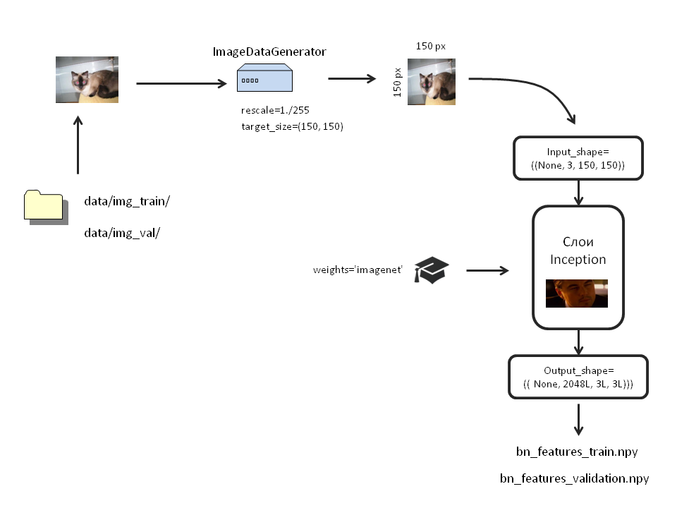
The Keras library has several prepared neural networks.
Model Argument List
include_top: to include or not to include the upper part of the network, which is a fully connected layer with 1000 outputs.
We don't need it, so we set: include_top = False;
weights : load / do not load trained weights. If None, the weights are initialized randomly. If imagenet, weights loaded with ImageNet data will be loaded.
In our model, weights are needed, so weights = "imagenet";
input_tensor : this argument is convenient if we use the Input layer for our model.
We will not touch it.
input_shape : in this argument we set the size of our image. It is indicated if the upper layer is detached (include_top = False). If we loaded the model with the top layer, one hundred image size should be only (3, 299, 299).
We removed the top layer and want to analyze smaller images (3, 150, 150). Therefore, show: input_shape = ()
Create our model:
inc_model=InceptionV3(include_top=False, weights='imagenet', input_shape=((3, 150, 150))) Now we will augment the data. For this Keras provides the so-called ImageDataGenerator. They will take images directly from the folders and carry out all the necessary transformations on them.
Pictures of each class must be in separate folders. In order for us not to load RAM with images, we transform them right before uploading to the network. For this we use the .flow_from_directory method. Create separate generators for training and test images:
bottleneck_datagen = ImageDataGenerator(rescale=1./255) #, train_generator = bottleneck_datagen.flow_from_directory('data/img_train/', target_size=(150, 150), batch_size=32, class_mode=None, shuffle=False) validation_generator = bottleneck_datagen.flow_from_directory('data/img_val/', target_size=(150, 150), batch_size=32, class_mode=None, shuffle=False) I want to highlight an important point. We specified shuffle = False . That is, images from different classes will not be mixed. First, there will be images from the first folder, and when they all end, from the second. Why it is needed, see later.
Run the augmented images through the trained Inception and save the output as numpy arrays:
bottleneck_features_train = inc_model.predict_generator(train_generator, 2000) np.save(open('bottleneck_features/bn_features_train.npy', 'wb'), bottleneck_features_train) bottleneck_features_validation = inc_model.predict_generator(validation_generator, 2000) np.save(open('bottleneck_features/bn_features_validation.npy', 'wb'), bottleneck_features_validation) The process will take some time.
3. Create the upper part of the model, load the data into it, save it:
Scheme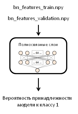
In the original post, the author used one network layer with 256 neurons, however I will use two layers with 64 neurons each and a Dropout layer with a value of 0.5. I was forced to make this change due to the fact that when I trained the finished model (which we will do in the next step), my computer would hang and reboot.
Load the arrays:
train_data = np.load(open('bottleneck_features_and_weights/bn_features_train.npy', 'rb')) train_labels = np.array([0] * 1000 + [1] * 1000) validation_data = np.load(open('bottleneck_features_and_weights/bn_features_validation.npy', 'rb')) validation_labels = np.array([0] * 1000 + [1] * 1000) Please note, earlier we specified shuffle = False . And now we can easily specify the labels . Since in each class we have 2000 images and all the images were received in turn, we will have 1000 zeros and 1000 units for training and for test samples.
Create a model of the FFN network, compile it:
fc_model = Sequential() fc_model.add(Flatten(input_shape=train_data.shape[1:])) fc_model.add(Dense(64, activation='relu', name='dense_one')) fc_model.add(Dropout(0.5, name='dropout_one')) fc_model.add(Dense(64, activation='relu', name='dense_two')) fc_model.add(Dropout(0.5, name='dropout_two')) fc_model.add(Dense(1, activation='sigmoid', name='output')) fc_model.compile(optimizer='rmsprop', loss='binary_crossentropy', metrics=['accuracy']) Let's load our arrays into it:
fc_model.fit(train_data, train_labels, nb_epoch=50, batch_size=32, validation_data=(validation_data, validation_labels)) fc_model.save_weights('bottleneck_features_and_weights/fc_inception_cats_dogs_250.hdf5') # Now we load data not from folders, so we use the usual fit method.
The learning process will be indecently fast. Each epoch took 1 sec from me:
Train on 2000 samples, validate on 2000 samples Epoch 1/50 2000/2000 [==============================] - 1s - loss: 2.4588 - acc: 0.8025 - val_loss: 0.7950 - val_acc: 0.9375 Epoch 2/50 2000/2000 [==============================] - 1s - loss: 1.3332 - acc: 0.8870 - val_loss: 0.9330 - val_acc: 0.9160 … Epoch 48/50 2000/2000 [==============================] - 1s - loss: 0.1096 - acc: 0.9880 - val_loss: 0.5496 - val_acc: 0.9595 Epoch 49/50 2000/2000 [==============================] - 1s - loss: 0.1100 - acc: 0.9875 - val_loss: 0.5600 - val_acc: 0.9560 Epoch 50/50 2000/2000 [==============================] - 1s - loss: 0.0850 - acc: 0.9895 - val_loss: 0.5674 - val_acc: 0.9565 We estimate the accuracy of the model:
fc_model.evaluate(validation_data, validation_labels) [0.56735104312408047, 0.95650000000000002]
Our model is doing its job well. But it takes only numpy arrays. It does not suit us. In order to get a full-fledged model that accepts images as input, we will connect our two models and train them again.
4. Create the final model, load the augmented data into it, save the weights:
Scheme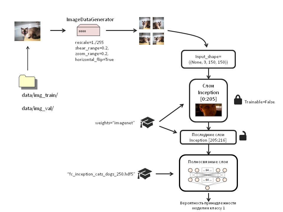
weights_filename='bottleneck_features_and_weights/fc_inception_cats_dogs_250.hdf5' x = Flatten()(inc_model.output) x = Dense(64, activation='relu', name='dense_one')(x) x = Dropout(0.5, name='dropout_one')(x) x = Dense(64, activation='relu', name='dense_two')(x) x = Dropout(0.5, name='dropout_two')(x) top_model=Dense(1, activation='sigmoid', name='output')(x) model = Model(input=inc_model.input, output=top_model) Load weights into it:
weights_filename='bottleneck_features_and_weights/fc_inception_cats_dogs_250.hdf5' model.load_weights(weights_filename, by_name=True) To be honest, I did not notice any difference between the effectiveness of training the model with or without loading weights. But I left this section because it describes how to load weights into certain layers by name (by_name = True).
Block from 1 to 205 layers Inception:
for layer in inc_model.layers[:205]: layer.trainable = False Compile the model:
model.compile(loss='binary_crossentropy', optimizer=SGD(lr=1e-4, momentum=0.9), #optimizer='rmsprop', metrics=['accuracy']) Notice that the first time we trained fully connected layers from .npy arrays, we used the RMSprop optimizer. Now, to tune the model, we use the Stochastic Gradient Descent. This is done in order to prevent too pronounced updates to the already trained weights.
Let us make sure that in the learning process only the weights with the highest accuracy on the test sample are saved:
filepath="new_model_weights/weights-improvement-{epoch:02d}-{val_acc:.2f}.hdf5" checkpoint = ModelCheckpoint(filepath, monitor='val_acc', verbose=1, save_best_only=True, mode='max') callbacks_list = [checkpoint] Create new image generators for learning the full model. We will transform only the training sample. Test will not touch.
train_datagen = ImageDataGenerator( rescale=1./255, shear_range=0.2, zoom_range=0.2, horizontal_flip=True) test_datagen = ImageDataGenerator(rescale=1./255) train_generator = train_datagen.flow_from_directory( 'data/img_train/', target_size=(150, 150), batch_size=32, class_mode='binary') validation_generator = test_datagen.flow_from_directory( 'data/img_val/', target_size=(150, 150), batch_size=32, class_mode='binary') pred_generator=test_datagen.flow_from_directory('data/img_val/', target_size=(150,150), batch_size=100, class_mode='binary') we use pred_generator later to demonstrate how the model works.
Load the images into the model:
model.fit_generator( train_generator, samples_per_epoch=2000, nb_epoch=200, validation_data=validation_generator, nb_val_samples=2000, callbacks=callbacks_list) We hear the noise of the cooler and wait ...
Epoch 1/200 1984/2000 [============================>.] - ETA: 0s - loss: 1.0814 - acc: 0.5640Epoch 00000: val_acc improved from -inf to 0.71750, saving model to new_model_weights/weights-improvement-00-0.72.hdf5 2000/2000 [==============================] - 224s - loss: 1.0814 - acc: 0.5640 - val_loss: 0.6016 - val_acc: 0.7175 Epoch 2/200 1984/2000 [============================>.] - ETA: 0s - loss: 0.8523 - acc: 0.6240Epoch 00001: val_acc improved from 0.71750 to 0.77200, saving model to new_model_weights/weights-improvement-01-0.77.hdf5 2000/2000 [==============================] - 215s - loss: 0.8511 - acc: 0.6240 - val_loss: 0.5403 - val_acc: 0.7720 … Epoch 199/200 1968/2000 [============================>.] - ETA: 1s - loss: 0.1439 - acc: 0.9385Epoch 00008: val_acc improved from 0.90650 to 0.91500, saving model to new_model_weights/weights-improvement-08-0.92.hdf5 2000/2000 [==============================] - 207s - loss: 0.1438 - acc: 0.9385 - val_loss: 0.2786 - val_acc: 0.9150 Epoch 200/200 1968/2000 [============================>.] - ETA: 1s - loss: 0.1444 - acc: 0.9350Epoch 00009: val_acc did not improve 2000/2000 [==============================] - 206s - loss: 0.1438 - acc: 0.9355 - val_loss: 0.3898 - val_acc: 0.8940 It took me 210-220 seconds for each epoch. 200 learning epochs took about 12 hours.
5. We estimate the accuracy of the model.
model.evaluate_generator(pred_generator, val_samples=100) [0.2364250123500824, 0.9100000262260437]
This is where the pred_generator came in handy . Please note, val_samples must match the batch_size value in the generator!
Accuracy 91.7%. Given the limitations of the sample, I dare to say that this is a good accuracy.
Illustrate the work of the model
Just look at the% correct answers and the magnitude of the error we are not interested. Let's see how many correct and incorrect answers were given by the model for each class:
imgs,labels=pred_generator.next() array_imgs=np.transpose(np.asarray([img_to_array(img) for img in imgs]),(0,2,1,3)) predictions=model.predict(imgs) rounded_pred=np.asarray([round(i) for i in predictions]) pred_generator.next () is a handy thing. It loads images into a variable and assigns labels.
The number of images of each class will be different with each generation:
pd.value_counts(labels) 0.0 51 1.0 49 dtype: int64 How many images of each class model predicted correctly?
pd.crosstab (labels, rounded_pred)
| Col_0 | 0.0 | 1.0 |
|---|---|---|
| Row_0 | ||
| 0.0 | 47 | four |
| 1.0 | eight | 41 |
For the model, 100 random images were uploaded: 51 images of cats and 49 dogs. Of the 51 cats, 47 recognized the model correctly. Of the 50 dogs, 41 were correctly recognized. The overall accuracy of the model on this narrow sample was 88%.
Let's see which photos were recognized incorrectly:
wrong=[im for im in zip(array_imgs, rounded_pred, labels, predictions) if im[1]!=im[2]] plt.figure(figsize=(12,12)) for ind, val in enumerate(wrong[:100]): plt.subplots_adjust(left=0, right=1, bottom=0, top=1, wspace = 0.2, hspace = 0.2) plt.subplot(5,5,ind+1) im=val[0] plt.axis('off') plt.text(120, 0, round(val[3], 2), fontsize=11, color='red') plt.text(0, 0, val[2], fontsize=11, color='blue') plt.imshow(np.transpose(im,(2,1,0))) 
Blue numbers are a true class of images. Red numbers are predicted by the model (if the red number is less than 0.5, the model considers that in the photo is a cat, if more than 0.5, then the dog). The more the number approaches zero, the more confident the network is that the cat is in front of it. Interestingly, many bugs with dog images contain small breeds or puppies.
Let's look at the first 20 images that the model predicted correctly:
right=[im for im in zip(array_imgs, rounded_pred, labels, predictions) if im[1]==im[2]] plt.figure(figsize=(12,12)) for ind, val in enumerate(right[:20]): plt.subplots_adjust(left=0, right=1, bottom=0, top=1, wspace = 0.2, hspace = 0.2) plt.subplot(5,5,ind+1) im=val[0] plt.axis('off') plt.text(120, 0, round(val[3], 2), fontsize=11, color='red') plt.text(0, 0, val[2], fontsize=11, color='blue') plt.imshow(np.transpose(im,(2,1,0))) 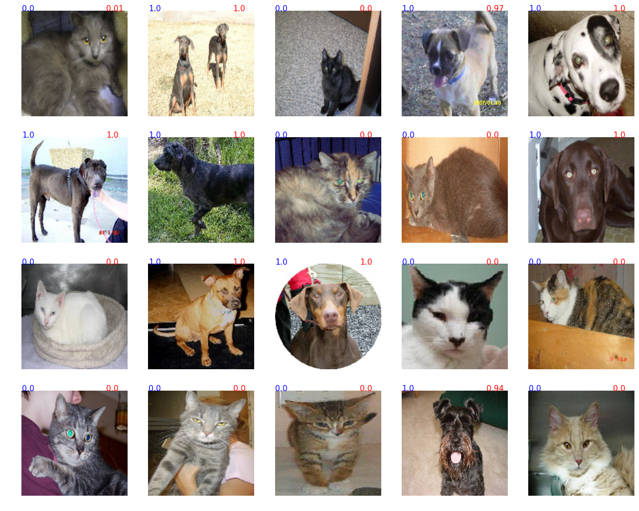
It can be seen that the model decently copes with the task of image recognition in relatively small samples.
I hope the post was helpful to you. I am pleased to hear your questions or suggestions.
Github Project
Source: https://habr.com/ru/post/321834/
All Articles