Heat equation in tensorflow

Hi, Habr! Some time ago I became interested in deep learning and began to slowly study tensorflow. While digging into tensorflow, I remembered my coursework on parallel programming, which I did that year in 4th year of university. The task there was formulated as follows:

Linear initial-boundary value problem for a two-dimensional heat equation:

$\ frac {\ partial u} {\ partial t} = \ sum \ limits _ {\ alpha = 1} ^ {2} \ frac {\ partial} {\ partial x_ \ alpha} \ left (k_ \ alpha \ frac {\ partial u} {\ partial x_ \ alpha} \ right) -u, \ quad x_ \ alpha \ in [0,1] \ quad (\ alpha = 1,2), \ t & gt; 0;$

$k_ \ alpha = \ begin {cases} 50, (x_1, x_2) \ in \ Delta ABC \\ 1, (x_1, x_2) \ notin \ Delta ABC \ end {cases}$

$(\ alpha = 1,2), \ A (0.2,0.5), \ B (0.7,0.2), \ C (0.5,0.8);$

$u (x_1, x_2, 0) = 0, \ u (0, x_2, t) = 1 - e ^ {- \ omega t}, \ u (1, x_2, t) = 0,$

$u (x_1,0, t) = 1 - e ^ {- \ omega t}, \ u (0, x_2, t) = 0, \ \ omega = 20.$

Although it would be better to call it the diffusion equation.
')
The task then needed to be solved by the finite difference method in an implicit scheme, using MPI for parallelization and the conjugate gradient method.

I am not an expert in numerical methods until I am an expert in tensorflow, but I already have experience. And I was eager to try to calculate urmata on a deep learning framework. The method of conjugate gradients to implement the second time is no longer interesting, but it is interesting to see how tensorflow will cope with the calculation and what difficulties will arise. This post is about what came of it.

Numerical algorithm

Define the grid:

$\ Omega = \ omega_ {x_1} \ times \ omega_ {x_2} \ times \ omega_t,$

$\ [\ omega_ {x_ \ alpha} = \ left \ {x _ {\ alpha, i_ \ alpha} = i_ \ alpha h, i_ \ alpha = 0, ..., N, h = \ frac {1} {N }, \ right \} \ \ alpha = 1,2, \]$

$\ [\ omega_t = \ left \ {t_j = j \ tau, j = 0, ..., N_t, \ tau = \ frac {t_ {max}} {N_t} \ right \}.$

Difference scheme:

To make it easier to paint, we introduce the operators:

$\ Delta_ {1} f_ {i, j} = \ frac {f_ {i + 1/2, j} - f_ {i-1/2, j}} {h},$

$\ Delta_ {2} f_ {i, j} = \ frac {f_ {i, j + 1/2} - f_ {i, j-1/2}} {h}.$

Explicit Difference Scheme:

$\ frac {u_ {i, j} ^ t - u_ {i, j} ^ {t-1}} {\ tau} = \ Delta_ {1} (k_ {i, j} \ Delta_ {1} u_ {i , j} ^ {t-1}) + \ Delta_ {2} (k_ {i, j} \ Delta_ {2} u_ {i, j} ^ {t-1}) - u_ {i, j} ^ t .$

In the case of an explicit difference scheme, the values of the function at the previous time point are used for the calculation and there is no need to solve the equation for values $u ^ t_ {i, j}$ . However, this scheme is less accurate and requires a significantly smaller time step.

Implicit difference scheme:

$\ frac {u_ {i, j} ^ t - u_ {i, j} ^ {t-1}} {\ tau} = \ Delta_ {1} (k_ {i, j} \ Delta_ {1} u_ {i , j} ^ t) + \ Delta_ {2} (k_ {i, j} \ Delta_ {2} u_ {i, j} ^ t) - u_ {i, j} ^ t,$

$\ frac {u_ {i, j} ^ t - u_ {i, j} ^ {t-1}} {\ tau} = \ Delta_ {1} (k_ {i, j} \ frac {u_ {i + 1 / 2, j} ^ t - u_ {i-1/2, j} ^ t} {h}) + \ Delta_ {2} (k_ {i, j} \ frac {u_ {i, j + 1/2 } ^ t - u_ {i, j-1/2} ^ t} {h}) - u_ {i, j} ^ t,$

$\ frac {u_ {i, j} ^ t - u_ {i, j} ^ {t-1}} {\ tau} = \ frac {k_ {i + 1/2, j} \ frac {u_ {i + 1, j} ^ t - u_ {i, j} ^ t} {h} - k_ {i-1/2, j} \ frac {u_ {i, j} ^ t - u_ {i-1/2, j} ^ t} {h}} {h} + \ frac {k_ {i, j + 1/2} \ frac {u_ {i, j + 1} ^ t - u_ {i, j} ^ t} { h} - k_ {i, j-1/2} \ frac {u_ {i, j} ^ t - u_ {i, j-1/2} ^ t} {h}} {h} - u_ {i, j} ^ t,$

$\ frac {u_ {i, j} ^ t - u_ {i, j} ^ {t-1}} {\ tau} = \ frac {k_ {i + 1/2, j} u_ {i + 1, j } ^ t - u_ {i, j} ^ t - k_ {i-1/2, j} u_ {i, j} ^ t - u_ {i-1/2, j} ^ t + k_ {i, j +1/2} u_ {i, j + 1} ^ t - u_ {i, j} ^ t - k_ {i, j-1/2} u_ {i, j} ^ t - u_ {i, j- 1/2} ^ t} {h ^ 2} - u_ {i, j} ^ t.$

Transfer to the left side everything related to $u ^ t$ , and to the right $u ^ {t-1}$ and multiply by $\ tau$ :

$(1 + \ frac {\ tau} {h ^ 2} (k_ {i + 1/2, j} + k_ {i-1/2, j} + k_ {i, j + 1/2} + k_ { i, j-1/2}) + \ tau) u_ {i, j} ^ t - \\ - \ frac {\ tau} {h ^ 2} (k_ {i + 1/2, j} u_ {i + 1, j} ^ t + k_ {i-1/2, j} u ^ t_ {i-1, j} + k_ {i, j + 1/2} u ^ t_ {i, j + 1} + k_ {i, j-1/2} u ^ t_ {i, j-1}) = u ^ {t-1} _ {i, j}.$

In fact, we obtained an operator equation over the grid:

$Au ^ t = u ^ {t-1},$

what if to write down values $u ^ t$ in the nodes of the grid as an ordinary vector, is an ordinary system of linear equations ( $Ax = b$ ). The values at the previous time constant, as already calculated.
For convenience, we present the operator $A$ as the difference of two operators:

$A = D_A - (A ^ + + A ^ {-}),$

Where:

$D_A u ^ t = (1 + \ frac {\ tau} {h ^ 2} (k_ {i + 1/2, j} + k_ {i-1/2, j} + k_ {i, j + 1 / 2} + k_ {i, j-1/2}) + \ tau) u ^ t_ {i, j},$

$(A ^ + + A ^ {-}) u ^ t = \ frac {\ tau} {h ^ 2} (k_ {i + 1/2, j} u ^ t_ {i + 1, j} + k_ { i-1/2, j} u ^ t_ {i-1, j} + k_ {i, j + 1/2} u ^ t_ {i, j + 1} + k_ {i, j-1/2} u ^ t_ {i, j-1}).$

Replacing $u ^ t$ to our assessment $\ hat {u} ^ t$ , we write the error functional:

$r = A \ hat {u} ^ t - u ^ {t-1} = (D_A - A ^ + - A ^ {-}) \ hat {u} ^ t - u ^ {t-1},$

$L = \ sum r_ {i, j} ^ 2.$

Where $r_ {i, j}$ - error in the grid nodes.

We will iteratively minimize the error functional using a gradient.

As a result, the task has been reduced to the multiplication of tensors and gradient descent, and this is exactly what tensorflow was intended for.

Implementation at tensorflow

Briefly about tensorflow

In tensorflow, the computation graph is first constructed. Resources under the graph are allocated inside tf.Session . Graph nodes are operations on data. The cells for the input data in the graph are tf.placeholder . To execute a graph, you need to run the run method on the session object, passing in it the operation of interest and input data for placeholders. The run method returns the result of the operation and can also change the values inside tf.Variable within the session.

tensorflow itself is able to build graphs of operations that implement the backpropagation of a gradient, provided that the original graph contains only operations for which the gradient is implemented (not everyone yet).

Code:

First is the initialization code. Here we make all the preliminary operations and consider everything that can be calculated in advance.

Initialization

#  import numpy as np import pandas as pd import tensorflow as tf import matplotlib.pyplot as plt import matplotlib from matplotlib.animation import FuncAnimation from matplotlib import cm import seaborn #    ,   #     class HeatEquation(): def __init__(self, nxy, tmax, nt, k, f, u0, u0yt, u1yt, ux0t, ux1t): self._nxy = nxy #    x, y self._tmax = tmax #   self._nt = nt #    self._k = k #  k self._f = f #  f self._u0 = u0 #   #   self._u0yt = u0yt self._u1yt = u1yt self._ux0t = ux0t self._ux1t = ux1t #       self._h = h = np.array(1./nxy) self._ht = ht = np.array(tmax/nt) print("ht/h/h:", ht/h/h) self._xs = xs = np.linspace(0., 1., nxy + 1) self._ys = ys = np.linspace(0., 1., nxy + 1) self._ts = ts = np.linspace(0., tmax, nt + 1) from itertools import product #       self._vs = vs = np.array(list(product(xs, ys)), dtype=np.float64) #   self._vcs = vsc = np.array(list(product(xs[1:-1], ys[1:-1])), dtype=np.float64) #      k vkxs = np.array(list(product((xs+h/2)[:-1], ys)), dtype=np.float64) # k_i+0.5,j vkys = np.array(list(product(xs, (ys+h/2)[:-1])), dtype=np.float64) # k_i ,j+0.5 #    k self._kxs = kxs = k(vkxs).reshape((nxy,nxy+1)) self._kys = kys = k(vkys).reshape((nxy+1,nxy)) #   D_A D_A = np.zeros((nxy+1, nxy+1)) D_A[0:nxy+1,0:nxy+0] += kys D_A[0:nxy+1,1:nxy+1] += kys D_A[0:nxy+0,0:nxy+1] += kxs D_A[1:nxy+1,0:nxy+1] += kxs self._D_A = D_A = 1 + ht/h/h*D_A[1:nxy,1:nxy] + ht # ,    self._U_shape = (nxy+1, nxy+1, nt+1) #        , #    ,     self._U = np.zeros(self._U_shape) #       self._U[:,:,0] = u0(vs).reshape(self._U_shape[:-1])

$\ tau$ and $h$ should be taken such that $\ frac {\ tau} {h ^ 2}$ was small, preferably at least <1, especially when using "nonsmooth" functions.

The method that builds the equation graph:

Computation graph

 # ,   def build_graph(self, learning_rate): def reset_graph(): if 'sess' in globals() and sess: sess.close() tf.reset_default_graph() reset_graph() nxy = self._nxy #   kxs_ = tf.placeholder_with_default(self._kxs, (nxy,nxy+1)) kys_ = tf.placeholder_with_default(self._kys, (nxy+1,nxy)) D_A_ = tf.placeholder_with_default(self._D_A, self._D_A.shape) U_prev_ = tf.placeholder(tf.float64, (nxy+1, nxy+1), name="U_t-1") f_ = tf.placeholder(tf.float64, (nxy-1, nxy-1), name="f") #      ,     U_ = tf.Variable(U_prev_, trainable=True, name="U_t", dtype=tf.float64) #   def s(tensor, frm): return tf.slice(tensor, frm, (nxy-1, nxy-1)) #    A+_A-  u Ap_Am_U_ = s(U_, (0, 1))*s(self._kxs, (0, 1)) Ap_Am_U_ += s(U_, (2, 1))*s(self._kxs, (1, 1)) Ap_Am_U_ += s(U_, (1, 0))*s(self._kys, (1, 0)) Ap_Am_U_ += s(U_, (1, 2))*s(self._kys, (1, 1)) Ap_Am_U_ *= self._ht/self._h/self._h #  res = D_A_*s(U_,(1, 1)) - Ap_Am_U_ - s(U_prev_, (1, 1)) - self._ht*f_ #  ,    loss = tf.reduce_sum(tf.square(res), name="loss_res") #         u0yt_ = None u1yt_ = None ux0t_ = None ux1t_ = None if self._u0yt: u0yt_ = tf.placeholder(tf.float64, (nxy+1,), name="u0yt") loss += tf.reduce_sum(tf.square(tf.slice(U_, (0, 0), (1, nxy+1)) - tf.reshape(u0yt_, (1, nxy+1))), name="loss_u0yt") if self._u1yt: u1yt_ = tf.placeholder(tf.float64, (nxy+1,), name="u1yt") loss += tf.reduce_sum(tf.square(tf.slice(U_, (nxy, 0), (1, nxy+1)) - tf.reshape(u1yt_, (1, nxy+1))), name="loss_u1yt") if self._ux0t: ux0t_ = tf.placeholder(tf.float64, (nxy+1,), name="ux0t") loss += tf.reduce_sum(tf.square(tf.slice(U_, (0, 0), (nxy+1, 1)) - tf.reshape(ux0t_, (nxy+1, 1))), name="loss_ux0t") if self._ux1t: ux1t_ = tf.placeholder(tf.float64, (nxy+1,), name="ux1t") loss += tf.reduce_sum(tf.square(tf.slice(U_, (0, nxy), (nxy+1, 1)) - tf.reshape(ux1t_, (nxy+1, 1))), name="loss_ux1t") #  ,        , #   ,    loss /= (nxy+1)*(nxy+1) #    train_step = tf.train.AdamOptimizer(learning_rate, 0.7, 0.97).minimize(loss) #     ,    self.g = dict( U_prev = U_prev_, f = f_, u0yt = u0yt_, u1yt = u1yt_, ux0t = ux0t_, ux1t = ux1t_, U = U_, res = res, loss = loss, train_step = train_step ) return self.g

In an amicable way, it was necessary to consider the values of the function at the edges as given and optimize the values of the function only in the inner region, but with this there were problems. There was no way to make only a part of the tensor optimized, and the gradient of the tensor does not have a gradient written at the moment of writing the post. One could try slyly tinkering on the edges or write your own optimizer. But simply adding the difference at the edges of the function values and the boundary conditions in the error functional works well.

It should be noted that the method with the adaptive moment proved to be the best, let the error functional and quadratic.

Calculation of the function : at each moment of time we do several optimization iterations, until we exceed maxiter or the error is less than eps, save and proceed to the next moment.

Calculation

 def train_graph(self, eps, maxiter, miniter): g = self.g losses = [] #    with tf.Session() as sess: #       sess.run(tf.global_variables_initializer(), feed_dict=self._get_graph_feed(0)) for t_i, t in enumerate(self._ts[1:]): t_i += 1 losses_t = [] losses.append(losses_t) d = self._get_graph_feed(t_i) p_loss = float("inf") for i in range(maxiter): #     #    u,   _, self._U[:,:,t_i], loss = sess.run([g["train_step"], g["U"], g["loss"]], feed_dict=d) losses_t.append(loss) if i > miniter and abs(p_loss - loss) < eps: p_loss = loss break p_loss = loss print('#', end="") return self._U, losses

Run:

Startup code

 tmax = 0.5 nxy = 100 nt = 10000 A = np.array([0.2, 0.5]) B = np.array([0.7, 0.2]) C = np.array([0.5, 0.8]) k1 = 1.0 k2 = 50.0 omega = 20 #     def triang(v, k1, k2, A, B, C): v_ = v.copy() k = k1*np.ones([v.shape[0]]) v_ = v - A B_ = B - A C_ = C - A m = (v_[:, 0]*B_[1] - v_[:, 1]*B_[0]) / (C_[0]*B_[1] - C_[1]*B_[0]) l = (v_[:, 0] - m*C_[0]) / B_[0] inside = (m > 0.) * (l > 0.) * (m + l < 1.0) k[inside] = k2 return k # 0.0 def f(v, t): return 0*triang(v, h0, h1, A, B, C) # 0.0 def u0(v): return 0*triang(v, t1, t2, A, B, C) #   def u0ytb(t, ys): return 1 - np.exp(-omega*np.ones(ys.shape[0])*t) def ux0tb(t, xs): return 1 - np.exp(-omega*np.ones(xs.shape[0])*t) def u1ytb(t, ys): return 0.*np.ones(ys.shape[0]) def ux1tb(t, xs): return 0.*np.ones(xs.shape[0]) #     eq = HeatEquation(nxy, tmax, nt, lambda x: triang(x, k1, k2, A, B, C), f, u0, u0ytb, u1ytb, ux0tb, ux1tb) _ = eq.build_graph(0.001) U, losses = eq.train_graph(1e-6, 100, 1)

results

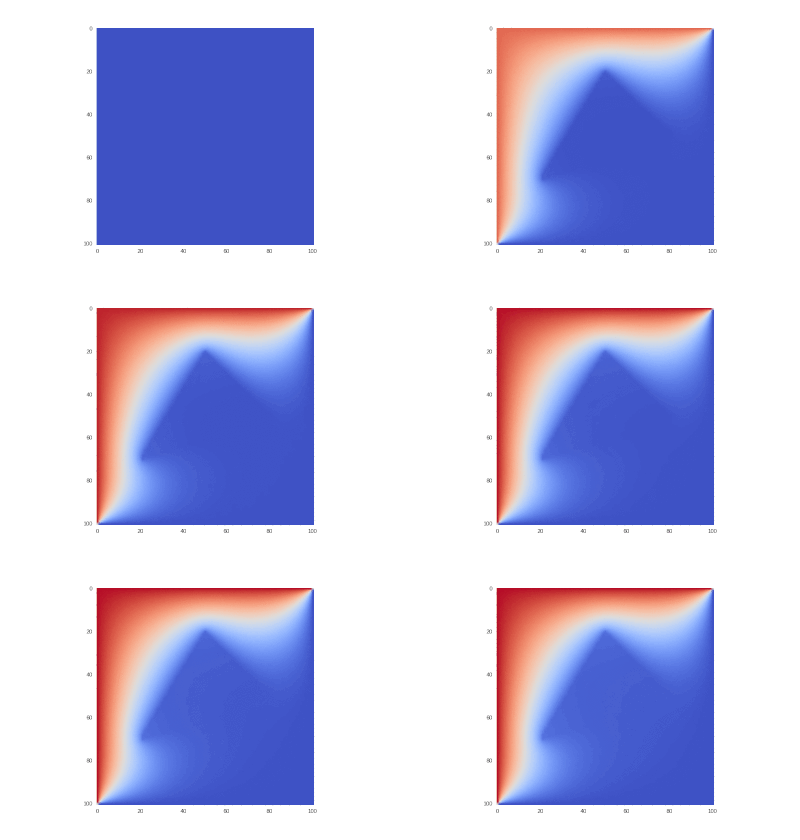
Original condition:

Hidden text

Condition as original, but without $-u$ in the equation:

Hidden text

$\ frac {\ partial u} {\ partial t} = \ sum \ limits _ {\ alpha = 1} ^ {2} \ frac {\ partial} {\ partial x_ \ alpha} \ left (k_ \ alpha \ frac {\ partial u} {\ partial x_ \ alpha} \ right), \ quad x_ \ alpha \ in [0,1] \ quad (\ alpha = 1,2), \ t & gt; 0;$

$k_ \ alpha = \ begin {cases} 50, (x_1, x_2) \ in \ Delta ABC \\ 1, (x_1, x_2) \ notin \ Delta ABC \ end {cases}$

$u (x_1, x_2, 0) = 0, \ u (0, x_2, t) = 1 - e ^ {- \ omega t}, \ u (1, x_2, t) = 0,$

$u (x_1,0, t) = 1 - e ^ {- \ omega t}, \ u (0, x_2, t) = 0, \ \ omega = 20.$

What is easily corrected in the code:

 #   __init__ self._D_A = D_A = 1 + ht/h/h*D_A[1:nxy,1:nxy]

There is almost no difference, because derivatives have larger orders than the function itself.

Further everywhere:

$\ frac {\ partial u} {\ partial t} = \ sum \ limits _ {\ alpha = 1} ^ {2} \ frac {\ partial} {\ partial x_ \ alpha} \ left (k_ \ alpha \ frac {\ partial u} {\ partial x_ \ alpha} \ right) + f, \ quad x_ \ alpha \ in [0,1] \ quad (\ alpha = 1,2), \ t & gt; 0;$

Condition with one heating edge:

Hidden text

$k_ \ alpha = \ begin {cases} 10, (x_1, x_2) \ in \ Delta ABC \\ 1, (x_1, x_2) \ notin \ Delta ABC \ end {cases}$

$f (x_1, x_2, t) = 0,$

$u (x_1, x_2, 0) = 0, \ u (0, x_2, t) = 1 - e ^ {- \ omega t}, \ u (1, x_2, t) = 0,$

$u (x_1,0, t) = 0, \ u (0, x_2, t) = 0, \ \ omega = 20.$

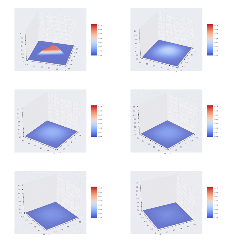
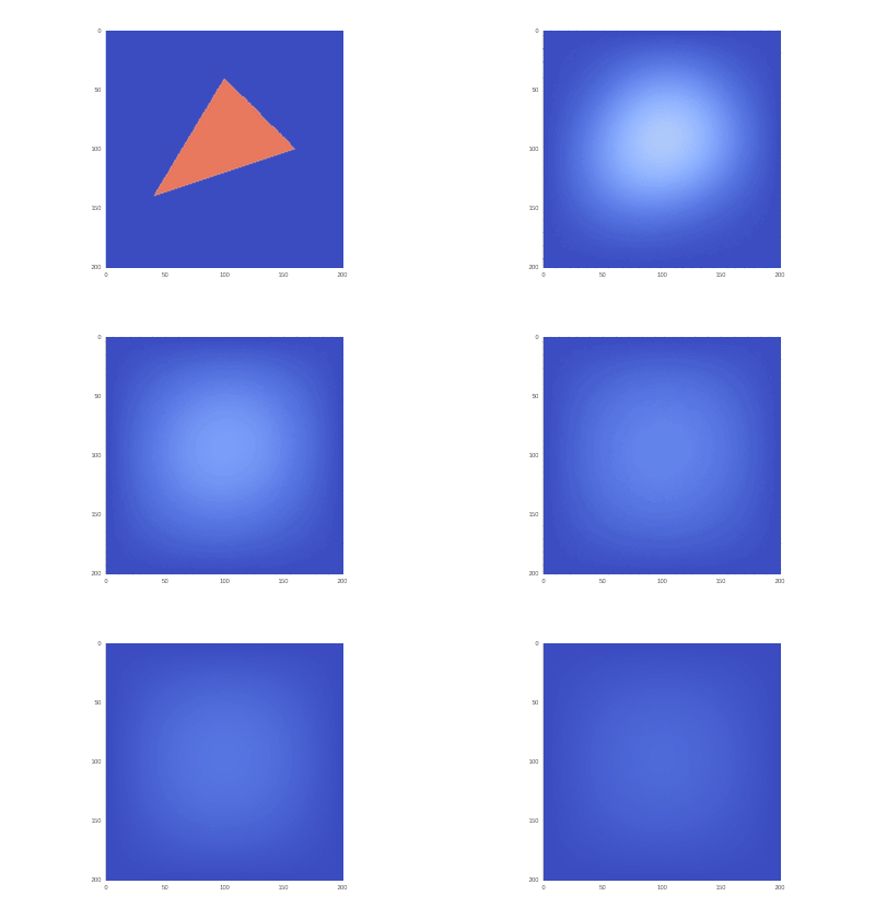
The condition with the cooling of the initially heated area:

Hidden text

$k_ \ alpha = 1,$

$f (x_1, x_2, t) = 0,$

$u (x_1, x_2, 0) = \ begin {cases} 0.1, (x_1, x_2) \ in \ Delta ABC \\ 0, (x_1, x_2) \ notin \ Delta ABC \ end {cases}$

$u (0, x_2, t) = 0, \ u (1, x_2, t) = 0,$

$u (x_1,0, t) = 0, \ u (0, x_2, t) = 0.$

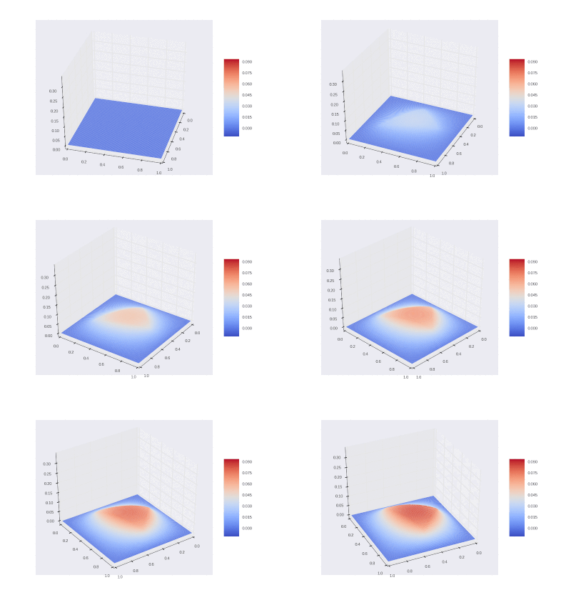
The condition with the inclusion of heating in the area:

Hidden text

$k_ \ alpha = \ begin {cases} 2, (x_1, x_2) \ in \ Delta ABC \\ 10, (x_1, x_2) \ notin \ Delta ABC \ end {cases}$

$f (x_1, x_2, t) = \ begin {cases} 10, (x_1, x_2) \ in \ Delta ABC \\ 0, (x_1, x_2) \ notin \ Delta ABC \ end {cases}$

$u (x_1, x_2, 0) = 0, \ u (0, x_2, t) = 0, \ u (1, x_2, t) = 0,$

$u (x_1,0, t) = 0, \ u (0, x_2, t) = 0.$

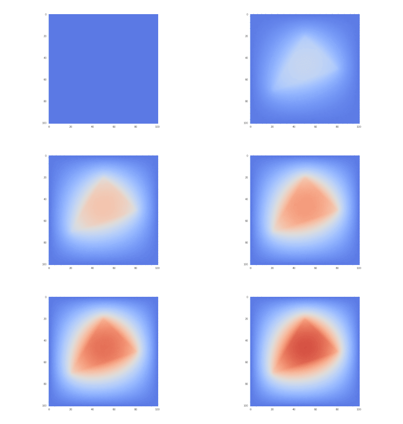
Drawing gifs

3D gif drawing function:

3d gif

In the main class, add a method that returns U in the form of pandas.DataFrame

 def get_U_as_df(self, step=1): nxyp = self._nxy + 1 nxyp2 = nxyp**2 Uf = self._U.reshape((nxy+1)**2,-1)[:, ::step] data = np.hstack((self._vs, Uf)) df = pd.DataFrame(data, columns=["x","y"] + list(range(len(self._ts))[0::step])) return df

 def make_gif(Udf, fname): from mpl_toolkits.mplot3d import Axes3D from matplotlib.ticker import LinearLocator, FormatStrFormatter from scipy.interpolate import griddata fig = plt.figure(figsize=(10,7)) ts = list(Udf.columns[2:]) data = Udf #    ,    matplotlib x1 = np.linspace(data['x'].min(), data['x'].max(), len(data['x'].unique())) y1 = np.linspace(data['y'].min(), data['y'].max(), len(data['y'].unique())) x2, y2 = np.meshgrid(x1, y1) z2s = list(map(lambda x: griddata((data['x'], data['y']), data[x], (x2, y2), method='cubic'), ts)) zmax = np.max(np.max(data.iloc[:, 2:])) + 0.01 zmin = np.min(np.min(data.iloc[:, 2:])) - 0.01 plt.grid(True) ax = fig.gca(projection='3d') ax.view_init(35, 15) ax.set_zlim(zmin, zmax) ax.zaxis.set_major_locator(LinearLocator(10)) ax.zaxis.set_major_formatter(FormatStrFormatter('%.02f')) norm = matplotlib.colors.Normalize(vmin=zmin, vmax=zmax, clip=False) surf = ax.plot_surface(x2, y2, z2s[0], rstride=1, cstride=1, norm=norm, cmap=cm.coolwarm, linewidth=0., antialiased=True) fig.colorbar(surf, shrink=0.5, aspect=5) #       def update(t_i): label = 'timestep {0}'.format(t_i) ax.clear() print(label) surf = ax.plot_surface(x2, y2, z2s[t_i], rstride=1, cstride=1, norm=norm, cmap=cm.coolwarm, linewidth=0., antialiased=True) ax.view_init(35, 15+0.5*t_i) ax.set_zlim(zmin, zmax) return surf, #     anim = FuncAnimation(fig, update, frames=range(len(z2s)), interval=50) anim.save(fname, dpi=80, writer='imagemagick')

2D gif drawing function:

2d gif

 def make_2d_gif(U, fname, step=1): fig = plt.figure(figsize=(10,7)) zmax = np.max(np.max(U)) + 0.01 zmin = np.min(np.min(U)) - 0.01 norm = matplotlib.colors.Normalize(vmin=zmin, vmax=zmax, clip=False) im=plt.imshow(U[:,:,0], interpolation='bilinear', cmap=cm.coolwarm, norm=norm) plt.grid(False) nst = U.shape[2] // step #       def update(i): im.set_array(U[:,:,i*step]) return im #     anim = FuncAnimation(fig, update, frames=range(nst), interval=50) anim.save(fname, dpi=80, writer='imagemagick')

Total

It should be noted that the original condition without using a GPU was considered 4m 26s, and using a GPU 2m 11s. For large points, the gap grows. However, not all operations in the resulting graph are GPU-compatible.

Machine Specifications:

Intel Core i7 6700HQ 2600 MHz,
NVIDIA GeForce GTX 960M.

You can see what operations are performed on what with the following code:

Hidden text

 #    def check_metadata_partitions_graph(self): g = self.g d = self._get_graph_feed(1) with tf.Session() as sess: sess.run(tf.global_variables_initializer(), feed_dict=d) options = tf.RunOptions(output_partition_graphs=True) metadata = tf.RunMetadata() c_val = sess.run(g["train_step"], feed_dict=d, options=options, run_metadata=metadata) print(metadata.partition_graphs)

It was an interesting experience. Tensorflow showed itself well for this task. Maybe even this approach will get some kind of application - it is more pleasant to write code on python than on C / C ++, and with the development of tensorflow it will become even easier.

Thanks for attention!

References

- Bakhvalov N. S., Zhidkov N. P., G. M. Kobelkov Numerical Methods , 2011

Source: https://habr.com/ru/post/321734/

All Articles

Heat equation in tensorflow

Numerical algorithm

Implementation at tensorflow

Briefly about tensorflow

Code:

results

Drawing gifs

Total

References

More articles: