How to stop guessing and start counting
Hello everyone, my name is Chudinov Denis and today we will look for mathematics in web analytics.
Traffic, of all physical phenomena, is rather complex from the point of view of the nature of the process, since, as far as I know, no one has yet formulated mathematical laws describing traffic. Nevertheless, we will try to apply the elementary methods of probability theory and mathematical statistics to formalize and evaluate the likelihood of our judgments.
Truth often remains fundamentally unattainable. Conducting research, we still encounter questions that can not be given a definite and reliable answer.
But is it bad?
Losing the opportunity to argue , we always reserve the right to evaluate . This loophole, however, does not allow us to touch the truth, but it allows us to get closer to it. Another thing is that people unknowingly or malicious intent regularly go the other way, moving away from the truth.
I can not keep myself from the pleasure for a moment to dive into the history of this issue.
')
One of the most important skills in mathematics is the art of inaccurate computing.
The beginning of a systematic study of problems related to mass random phenomena, and the emergence of the corresponding mathematical apparatus belong to the XVII century. Galileo tried to investigate the errors of physical measurements and estimate their probability.
For the whole of the XVIII and the beginning of the XIX century, the rapid development of the theory of probability and its widespread fascination are characteristic. The theory of probability becomes a “fashionable” science. It is beginning to be applied not only where this application is legitimate, but also where it is not justified in any way. This period is characterized by numerous attempts to apply probability theory to the study of social phenomena, to the so-called "moral" or "moral" sciences. Appeared work on issues of justice, history, politics, even theology, which used the apparatus of the theory of probability. For all these pseudo-scientific studies, an extremely simplified, mechanistic approach to the social phenomena considered in them is characteristic. Some arbitrarily set probabilities rely on the basis of reasoning (for example, when considering issues of legal proceedings, the propensity of every person to be truth or lie is estimated by some constant, the same probability for all people), and then the social problem is solved as a simple arithmetic problem. Naturally, all such attempts were doomed to failure and could not play a positive role in the development of science. On the contrary, their indirect result was the fact that in about the 20s – 30s of the 19th century in Western Europe, the widespread fascination with probability theory was replaced by disappointment and skepticism. Probability theory began to be viewed as a dubious, second-rate science, a kind of mathematical entertainment, hardly worthy of serious study. Go
At this point, it is necessary to pause and note that at that time, probability theory and mathematical statistics did not look at all like they do now.
It was at the beginning of the 19th century that the famous Petersburg Mathematical School was created in Russia, by whose works the theory of probability was put on a solid logical and mathematical basis and made a reliable, accurate and effective method of knowledge. Since the appearance of this school, the development of the theory of probability has already been closely associated with the work of Russians, and later of Soviet scientists.
As a tribute, I will give their surnames, and you can recall them (if you ever did a terver and matstat) how well their names entered these sciences.
V.Ya. Bunyakovsky, P.L. Chebyshev, A.A. Markov, A.M. Lyapunov and S.N. Bernstein, A.Ya. Khinchin, A.N. Kolmogorov, V.I. Romanovsky, N.V. Smirnov E.E. Slutsky, B.V. Gnedenko and others.
So, before we return to our question, let me remind you of the basics, without which it would be difficult for us to move on.
An event is a fact that occurred or did not occur as a result of experience. For example:
Random variable - a value that as a result of experience takes on a value that was not known in advance. For example:
Take the experience of throwing an ordinary hexagon dice: an event is random and we cannot predict its result, that is, we can name the dropped face in advance.
The mathematical laws of the theory of probability are obtained by abstracting the real statistical laws inherent in mass random phenomena. The presence of these patterns is associated precisely with the mass character of the phenomena, that is, with the large number of homogeneous experiments performed.
The specific features of each individual random phenomenon have almost no effect on the average result of the mass of such phenomena: random deviations from the average are mutually leveled. It is this stability of averages that constitutes the physical content of the law of large numbers : with a very large number of random phenomena, their average result practically ceases to be random and can be predicted with a large degree of certainty.
Thus, even for completely random events, there are “stable” metrics. In the previous example, we can estimate how many points on average will fall on a hexagonal cube with a large number of tests. To do this, we will roll a die many times, sum up all the points and divide by the number of tests.
In the same way, knowing the history of visits to the site, we can predict the attendance on a particular day with good accuracy.
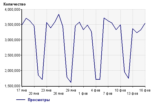
Let's take the open statistics of views from liveinternet for the site XXX
The question is: how “big” should there be a change on the site / in marketing, so that we can unequivocally (or rather, with a high degree of probability) say that this change affected the current metric?
Let's transfer the data to the table .
The current statistical material is a simple statistical series. Each element of the series is a sample of random variables of sufficiently large volume so that the essential features of the radiated distribution are revealed. In favor of this, we are told by the fact that on the graph one can see a certain periodic pattern.
We do not set ourselves the goal of solving the problem of aligning statistical series (that is, the task of finding a theoretical distribution curve expressing the features of a stat. Material), since searching for an analytical representation of the data obtained is a problem in itself and is solved, first of all, from considerations of physics process. Alas, the nature of traffic is so complex that we cannot theoretically describe it.
Moreover, to find the distribution law, we need an extensive stat. material, of the order of several hundred observations. Alas, we do not have this, but nevertheless, we can tentatively determine the most important numerical characteristics of a random variable: mathematical expectation , variance, and standard deviation .
Let us draw some conclusion about the physics of the process:
The traffic has a cyclical nature, so it is incorrect to compare different days of the week to each other. That is, if we want to find out how traffic behaves on Monday and how abnormal it is - we must compare the current Monday with all previous Mondays. Or take a longer period for research, for example a week, to get rid of periodic dependence.
In the table that I gave above, we take the last 5 media (that is, data on views for January 18, January 25, February 1, February 8 and February 15).
Estimate for the sample of these days the expectation and variance. It is known that the statistical average of a random variable tends to mat. waiting for the number of experiments, seeking to infinity. Alas, in practice we rarely have a large number of experiments, so we take into account the fact that our expectation is not accurate.
Given a sample of five elements:
3,703,900
3,577,305
3 329 611
3,538,719
3 325 899
Mat. expectation (it’s a statistical average): 3 495 087
Unbiased dispersion: 27,068,326,459
Standard deviation (square root of the variance): 164 525
Now the fun part. There is one such thing, called Chebyshev's inequality . In short, it claims that the random variable basically takes on a value close to its average. The same inequality gives a numerical estimate for this event:
Random variable with probability
What does it mean? Take k = 2 for our sample.
We obtain that the random variable falls in the interval (3 166 037, 3 824 137) with a probability of 75%.
Most often, k = 3 standard deviations are taken (the famous three-sigma rule), since in the worst case the accuracy is 88%.
This accuracy corresponds to the interval (3 001 512, 3 988 662).
The educated reader may note that the three sigma rule gives greater accuracy in some cases. Yes, this is so, in some cases, the accuracy of the assessment can be enhanced, but for this you need to know a little more about the nature of the distribution, and in this article we do not set ourselves such a task.
Before drawing any conclusions, let's graphically depict our results:
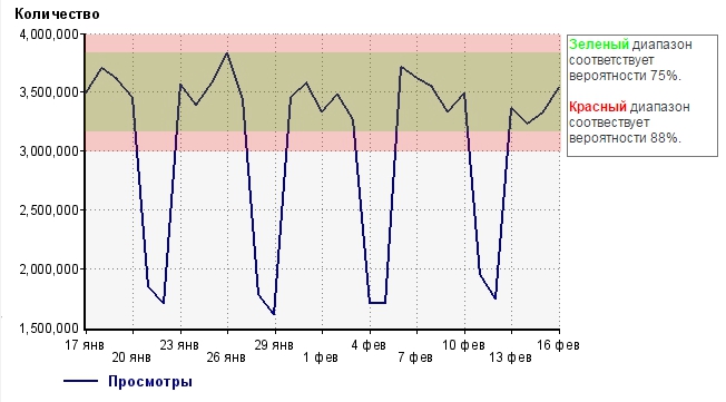
We found out that our random variable (the amount of site views during the day) with a probability of 75% will fall into the green range, and with a probability of 88% fall into the red range, if we do not drastically change anything in the nature of this value, that is, change the interface on the site or show marketing activity.
So what does this give us? To begin with, we will choose the border, which we will "believe." Traditionally, we take an interval of 3 sigma, that is, red.
It gives a window that deviates from the average by 14.1%.
If we conduct any experiment, for example, we perform an A / B test and measure the result next Wednesday (February 22), we can draw the following conclusions:
1. If the result of the experiment changed our indicator by more than 14.1% - most likely the experiment is successful.
2. If the result of the experiment changed our indicator by less than 14.1% - the experiment cannot be reliable, since the possible effect is within the limits of statistical error and is “blurred” by it. That is, even if the positive effect was - we can not reliably prove this at the current assessment.
What to do? Improve the estimate (take more observations, rather than 5, as I did), thus stretching the duration of the experiment.
Thanks for reading. I will be glad to criticism, suggestions and clarifications.
List of publications used in the post:
Traffic, of all physical phenomena, is rather complex from the point of view of the nature of the process, since, as far as I know, no one has yet formulated mathematical laws describing traffic. Nevertheless, we will try to apply the elementary methods of probability theory and mathematical statistics to formalize and evaluate the likelihood of our judgments.
Is it not a shame for a physicist, that is, a researcher and tester of nature, to look for evidence of truth in souls enslaved by custom? Mark Tullius Cicero, more than 2000 years ago
Truth often remains fundamentally unattainable. Conducting research, we still encounter questions that can not be given a definite and reliable answer.
But is it bad?
Losing the opportunity to argue , we always reserve the right to evaluate . This loophole, however, does not allow us to touch the truth, but it allows us to get closer to it. Another thing is that people unknowingly or malicious intent regularly go the other way, moving away from the truth.
I can not keep myself from the pleasure for a moment to dive into the history of this issue.
')
A tour of the history of probability theory and mathematical statistics
One of the most important skills in mathematics is the art of inaccurate computing.
The beginning of a systematic study of problems related to mass random phenomena, and the emergence of the corresponding mathematical apparatus belong to the XVII century. Galileo tried to investigate the errors of physical measurements and estimate their probability.
For the whole of the XVIII and the beginning of the XIX century, the rapid development of the theory of probability and its widespread fascination are characteristic. The theory of probability becomes a “fashionable” science. It is beginning to be applied not only where this application is legitimate, but also where it is not justified in any way. This period is characterized by numerous attempts to apply probability theory to the study of social phenomena, to the so-called "moral" or "moral" sciences. Appeared work on issues of justice, history, politics, even theology, which used the apparatus of the theory of probability. For all these pseudo-scientific studies, an extremely simplified, mechanistic approach to the social phenomena considered in them is characteristic. Some arbitrarily set probabilities rely on the basis of reasoning (for example, when considering issues of legal proceedings, the propensity of every person to be truth or lie is estimated by some constant, the same probability for all people), and then the social problem is solved as a simple arithmetic problem. Naturally, all such attempts were doomed to failure and could not play a positive role in the development of science. On the contrary, their indirect result was the fact that in about the 20s – 30s of the 19th century in Western Europe, the widespread fascination with probability theory was replaced by disappointment and skepticism. Probability theory began to be viewed as a dubious, second-rate science, a kind of mathematical entertainment, hardly worthy of serious study. Go
At this point, it is necessary to pause and note that at that time, probability theory and mathematical statistics did not look at all like they do now.
It was at the beginning of the 19th century that the famous Petersburg Mathematical School was created in Russia, by whose works the theory of probability was put on a solid logical and mathematical basis and made a reliable, accurate and effective method of knowledge. Since the appearance of this school, the development of the theory of probability has already been closely associated with the work of Russians, and later of Soviet scientists.
As a tribute, I will give their surnames, and you can recall them (if you ever did a terver and matstat) how well their names entered these sciences.
V.Ya. Bunyakovsky, P.L. Chebyshev, A.A. Markov, A.M. Lyapunov and S.N. Bernstein, A.Ya. Khinchin, A.N. Kolmogorov, V.I. Romanovsky, N.V. Smirnov E.E. Slutsky, B.V. Gnedenko and others.
So, before we return to our question, let me remind you of the basics, without which it would be difficult for us to move on.
A brief introduction to mathematical statistics
Denial of responsibility
I do not claim to be absolutely accurate and correct wording, as I am willing to sacrifice the severity of the description for the sake of convenience of explanation. At the end of the article, I suggest that attentive and more demanding readers find links to used literature and dive into the question themselves.
An event is a fact that occurred or did not occur as a result of experience. For example:
- When throwing the cube dropped 5 points.
- The user entered the site.
Random variable - a value that as a result of experience takes on a value that was not known in advance. For example:
- The number of points that fell on the cube.
- The sum of all the points that fell on the die for 1000 shots.
- The number of page views on the site during the day.
Take the experience of throwing an ordinary hexagon dice: an event is random and we cannot predict its result, that is, we can name the dropped face in advance.
The mathematical laws of the theory of probability are obtained by abstracting the real statistical laws inherent in mass random phenomena. The presence of these patterns is associated precisely with the mass character of the phenomena, that is, with the large number of homogeneous experiments performed.
The specific features of each individual random phenomenon have almost no effect on the average result of the mass of such phenomena: random deviations from the average are mutually leveled. It is this stability of averages that constitutes the physical content of the law of large numbers : with a very large number of random phenomena, their average result practically ceases to be random and can be predicted with a large degree of certainty.
Thus, even for completely random events, there are “stable” metrics. In the previous example, we can estimate how many points on average will fall on a hexagonal cube with a large number of tests. To do this, we will roll a die many times, sum up all the points and divide by the number of tests.
By the way, I suggest you check yourself and evaluate this number;) The answer is inside
An average of 3.5 points per die roll. And how many points on average falls when throwing three six-sided dice at the same time? Write your version in the comments!
In the same way, knowing the history of visits to the site, we can predict the attendance on a particular day with good accuracy.
Applying Mathematical Statistics to Web Analytics
Disclaimer # 2
As far as I know, no one does this in-depth analysis of traffic and web analytics of web analytics, so I don’t have the opportunity to refer to the experience of my colleagues. Therefore, keep in mind that this is the author's approach to the problem, does not claim to be true, is disapproved by anyone, at your own peril and risk.
Let's take the open statistics of views from liveinternet for the site XXX
The question is: how “big” should there be a change on the site / in marketing, so that we can unequivocally (or rather, with a high degree of probability) say that this change affected the current metric?
Let's transfer the data to the table .
The current statistical material is a simple statistical series. Each element of the series is a sample of random variables of sufficiently large volume so that the essential features of the radiated distribution are revealed. In favor of this, we are told by the fact that on the graph one can see a certain periodic pattern.
We do not set ourselves the goal of solving the problem of aligning statistical series (that is, the task of finding a theoretical distribution curve expressing the features of a stat. Material), since searching for an analytical representation of the data obtained is a problem in itself and is solved, first of all, from considerations of physics process. Alas, the nature of traffic is so complex that we cannot theoretically describe it.
Moreover, to find the distribution law, we need an extensive stat. material, of the order of several hundred observations. Alas, we do not have this, but nevertheless, we can tentatively determine the most important numerical characteristics of a random variable: mathematical expectation , variance, and standard deviation .
Let us draw some conclusion about the physics of the process:
The traffic has a cyclical nature, so it is incorrect to compare different days of the week to each other. That is, if we want to find out how traffic behaves on Monday and how abnormal it is - we must compare the current Monday with all previous Mondays. Or take a longer period for research, for example a week, to get rid of periodic dependence.
In the table that I gave above, we take the last 5 media (that is, data on views for January 18, January 25, February 1, February 8 and February 15).
Estimate for the sample of these days the expectation and variance. It is known that the statistical average of a random variable tends to mat. waiting for the number of experiments, seeking to infinity. Alas, in practice we rarely have a large number of experiments, so we take into account the fact that our expectation is not accurate.
Given a sample of five elements:
3,703,900
3,577,305
3 329 611
3,538,719
3 325 899
Mat. expectation (it’s a statistical average): 3 495 087
Unbiased dispersion: 27,068,326,459
Standard deviation (square root of the variance): 164 525
As I thought mate. waiting and dispersion
I am lazy enough to consider everything on my own, so I used one service that counted everything for me and wrote down the counting process.
Now the fun part. There is one such thing, called Chebyshev's inequality . In short, it claims that the random variable basically takes on a value close to its average. The same inequality gives a numerical estimate for this event:
Random variable with probability
will be in the interval (m-ks, m + ks), where k is a positive coefficient (k> 1), and s is the standard deviation.
What does it mean? Take k = 2 for our sample.
We obtain that the random variable falls in the interval (3 166 037, 3 824 137) with a probability of 75%.
Most often, k = 3 standard deviations are taken (the famous three-sigma rule), since in the worst case the accuracy is 88%.
This accuracy corresponds to the interval (3 001 512, 3 988 662).
The educated reader may note that the three sigma rule gives greater accuracy in some cases. Yes, this is so, in some cases, the accuracy of the assessment can be enhanced, but for this you need to know a little more about the nature of the distribution, and in this article we do not set ourselves such a task.
findings
Before drawing any conclusions, let's graphically depict our results:
We found out that our random variable (the amount of site views during the day) with a probability of 75% will fall into the green range, and with a probability of 88% fall into the red range, if we do not drastically change anything in the nature of this value, that is, change the interface on the site or show marketing activity.
So what does this give us? To begin with, we will choose the border, which we will "believe." Traditionally, we take an interval of 3 sigma, that is, red.
It gives a window that deviates from the average by 14.1%.
If we conduct any experiment, for example, we perform an A / B test and measure the result next Wednesday (February 22), we can draw the following conclusions:
1. If the result of the experiment changed our indicator by more than 14.1% - most likely the experiment is successful.
2. If the result of the experiment changed our indicator by less than 14.1% - the experiment cannot be reliable, since the possible effect is within the limits of statistical error and is “blurred” by it. That is, even if the positive effect was - we can not reliably prove this at the current assessment.
What to do? Improve the estimate (take more observations, rather than 5, as I did), thus stretching the duration of the experiment.
Thanks for reading. I will be glad to criticism, suggestions and clarifications.
List of publications used in the post:
- E.S. Wentzel "Theory of Probability" (1969, a very funny book, every second task about military affairs. Apparently affected by the imprint of the Cold War :)
- V.V. Svetozarov "Elementary processing of measurement results"
Source: https://habr.com/ru/post/321722/
All Articles