Neyrabayesovsky approach to machine learning problems. Lecture by Dmitry Vetrov in Yandex
With this post we complete a series of lectures with Data Fest. One of the central events of the conference was a report by Dmitry Vetrov , a professor at the Faculty of Computer Science of the National Research University Higher School of Economics. Dmitry is one of the most famous machine learning specialists in Russia and, since last year, has been working as a leading researcher at Yandex. In the report, he talks about the basics of the Bayesian approach and explains the advantages of this approach when using neural networks.
Under the cut - decoding and part of the slide.
Time a little, I will ride on tops. Those interested can watch the slides - there is a stricter conclusion and many beautiful and different formulas. Let's hope that will not be very boring.
What I will talk about. I will try to give a brief description of Bayesian methods, the Bayesian approach as a probability theory, as a machine learning problem. This approach was quite popular in the 90s and zero years - before the deep revolution started, caused by the triumphal procession of deep neural networks. For some time it seemed: why all these Bayes methods are needed, we have neural networks and so work fine. But as often happens, at some point it turned out that the advantages of the neural network and Bayesian approaches can be combined. First of all, due to the fact that the techniques of variational Bayes output appeared, and these models do not contradict each other, but on the contrary, they perfectly complement each other, reinforcing each other.
')
In a sense, I perceive it as a direction for the further development of modern machine learning and deep learning. It is important to understand that neural networks are not a panacea. They are just an important step in the right direction, but not the last step. I will try to talk about the next possible step in machine learning theory. And the next speaker, Sergey Bartunov, will try to engage in the deconstruction of the myth and in some sense continue the idea that in-depth training is not a panacea. But Sergey will approach this somewhat from the other side, will provide some more global view.

So what is the Bayesian approach? The whole approach is based on a single formula or theorem. Bayes theorem is given in mathematical and conceptual forms.
Key idea Suppose there is some unknown quantity that we would like to evaluate for some of its indirect manifestations. In this case, the unknown quantity is θ, and its indirect manifestation is y. Then you can use the Bayes theorem, which allows our initial ignorance or knowledge of an unknown quantity, a priori knowledge, to transform into a posteriori after observing some indirect characteristics, somehow indirectly characterizing the unknown quantity θ.
The key feature of the formula is that we input an a priori distribution that encodes our ignorance or our uncertainty about an unknown value, and that the output is also a distribution. This is a very important point. Not a point estimate, but a certain entity of the same format that was at the entrance. Due to this, it becomes possible, for example, to use the Bayesian inference, a posteriori distribution, as a priori in some new probabilistic model and, thus, to characterize a new unknown value from different sides by analyzing its various indirect manifestations. This is the first advantage due to which it is possible to obtain the extensibility property - or compositionability - of different probabilistic models, when we can build more complex ones from simple models.
The second interesting property. The simplest rule for summing the product of probabilities is: if we have a probabilistic model — in other words, a joint probability distribution for all variables arising in our problem — then, at least in theory, we can always construct any probabilistic forecast, predict the variable of interest U, knowing some observable variables O. In this case, there is a variable L, which we do not know and does not interest us. According to this formula, they are perfectly excluded from consideration.
For any combination of these three groups of variables, we can always construct such a conditional distribution, which will indicate how our ideas about the quantities U of interest to us have changed, if we have observed the O values supposedly related to U.

In fact, the widespread use of Bayes formulas gave birth to a second alternative approach to probability theory. There is a classic approach - often called frequency, phreakventist in the West - and there is an alternative Bayesian approach. Here is a brief table that I give in all my lectures and which shows the differences between the approaches. Naturally, they do not contradict each other. They rather complement each other. On this label you can see what they have in common and what are the differences.
The key difference is what is meant by a random variable. In frequency terms, we understand by a random variable a quantity, the value of which we cannot predict without appreciating any statistical patterns. Something with objective uncertainty is needed, while in the Bayesian approach the random variable is interpreted simply as a deterministic process. It can be fully predicted. Just in this deterministic process, we do not know part of the factors that influence the outcome. Since we do not know them, we cannot predict the outcome of the deterministic process. So, for us, this outcome looks like a random variable.
The simplest example is a coin flip. This is a classic random value, but we understand that the coin obeys the laws of classical mechanics and, in fact, knowing all the initial conditions — force, acceleration, coefficient of resistance of the medium, etc. — we could say for sure will fall: an eagle or tails.
If you think about it, the overwhelming majority of the quantities that we used to think of as random are actually random in the Bayesian sense. These are some deterministic processes, we just do not know part of the factors of these processes.
Since one may not know some factors, and the other - others, the concept of subjective uncertainty or subjective ignorance arises.
The rest is the direct difference between this interpretation. All values in the Bayesian approach can be interpreted as random. The apparatus of probability theory is applied to the distribution parameters of a random variable. In other words, the fact that in the classical approach is meaningless, in the Bayesian approach makes sense. The method of the statistical method, instead of the maximum likelihood method - Bayes theorem. Estimates are not point-like, but a kind of posterior distribution, allowing us to combine different probabilistic models. And unlike the frequency approach - theoretically justified for large n, and some prove, for example, when n tends to infinity - the Bayesian approach is true for any sample size, even if n = 0. Just in this case, the a posteriori distribution will coincide with the prior .

Simple illustration. A famous parable about blind wise men and an elephant, showing how a model can be hooked.
Let's imagine: given several blind sages and one elephant. The task is to estimate the mass of this elephant. Wise men know that they will now feel a certain animal. What exactly - do not know, but they have to evaluate the mass.
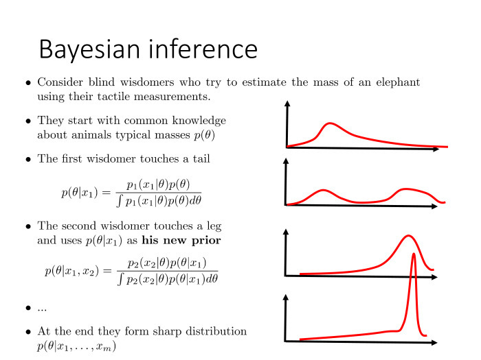
They all start by coding their ideas about the possible mass of an animal in the form of an a priori distribution, since now the distribution density can determine a simple measure of our ignorance about something. To encode this knowledge, we can simply use the apparatus of probability theory.
As far as sages are concerned, they know the characteristic masses of animals on planet Earth. Therefore, they get about this prior distribution.
The first sage comes up, feels the tail and concludes that, apparently, there is something snake-like or the tail of a large animal in front of him. Hence, in the process of his Bayesian inference, by combining the results of his representations, which can be expressed in the form of a probability partition p1, he obtains the posterior distribution p (θ) under the condition x = 1.
Then comes another sage who can not feel, but say, sniff. There is a completely different model. X2 is a value from a completely different domain, indirectly characterizing the mass of the animal. In the process of his Bayesian inference, he uses, as an a priori distribution, not the initial distribution from which everyone started, but the result of the output of the previous sage. Thus, we can combine two completely different dimensions, two sources of information, in one elegant probabilistic model.
And so, having done a series of measurements, we end up with a fairly sharp a posteriori distribution, an almost accurate estimate. We can already say with high accuracy what weight the animal had. This is an illustration of the third property - to extendibility, that is, the ability of the model to expand and hook all the time.
Another advantage of the Bayesian approach, already applied to machine learning, is regularization. By taking into account a priori preferences, we prevent the excessive adjustment of our parameters during the machine learning procedure and are thus able to cope with the effect of retraining. Some time ago, when the algorithms began to train on huge amounts of data, it was thought that the problem of retraining was removed from the agenda. But it was all about the fact that people were psychologically afraid to switch to giant-sized neural networks. Everyone started with small neural networks, and they, with giant training samples, did not really retrain. But as psychological fear disappeared, people began to use larger networks.
Two things have become obvious. For a start, the larger the network, the better it is in principle. Large networks work better than small ones. But large networks are starting to retrain. If we have a number of parameters - 100 million, then 1 billion objects are not a very large training sample, and we need to regularize the procedure of such machine learning.
The Bayesian approach provides an excellent opportunity to do this by introducing an a priori distribution on those parameters, on those neural network weights that are configured during the training procedure.
In particular, it turned out that such a popular heuristic regularization technique, such as drop out, is a special case, a rough approximation for Bayesian regularization. In fact, this is an attempt to make a Bayesian conclusion.
Finally, the third advantage is the ability to build a model with latent variables. About her more.

We have a motivating example - the main component method. The method is very simple - linear reduction of the dimension. We take a sample in space with a high dimension, build a covariance matrix, project it onto the main axis with the corresponding largest value. Here is what is geometrically shown here. And reduced the dimension of the space from 2 to 1, while maintaining the maximum dispersion contained in the sample.
The method is simple, allows the solution in an explicit form. But you can alternatively formulate differently, in terms of a probabilistic model.

Imagine that our data is arranged as follows: for each object there is its hidden representation in a space of small dimension. Here, it is labeled z. And we observe a linear function of this hidden representation in space with a higher dimension. We took a linear function and additionally added normal noise. Thus, we obtained x, high-dimensional data, according to which it is highly desirable for us to restore their low-dimensional representation.

Mathematically, it looks like this. We set a probabilistic model, which is the joint probability distribution for observable and hidden components, on x and z. The model is quite simple, the sample is characterized by the product of objects. The observable component of each object is determined by the hidden component; we are talking about a priori distribution on the hidden component. Both are normal distributions. We assume that in a small space the data is distributed a priori normally, and we observe a linear function of this data, which is noisy with normal noise.
We are given a sample, which is a high-dimensional representation. We know x, we do not know z, and our task is to find the parameter θ. θ is the V, σ² matrix and that's it.
This problem can be formulated in Bayesian language as a learning task with latent variables. To apply the usual maximum likelihood method, there is not enough knowledge of increasing z. It turns out that for this technique there is a standard approach based on the EM algorithm and various modifications. You can run an iterative process. The EM-step contains formulas describing what we are doing. It can theoretically be shown that the process is monotonous and is guaranteed to converge to a local extremum, but still.
The question arises: why do we need to use the iterative process, when we know that the problem is solved explicitly?
The answer is simple. To begin with - algorithmic complexity. The complexity of the analytical solution is O (nD²), while the complexity of one iteration of the EM algorithm is O (nDd).
If we mentally imagine that we are projecting a space of 1 million in space with a dimension of 10, and the EM algorithm converges iterations over one hundred, then our iterative scheme will work 1000 times faster than an explicit solution.
In addition, an important advantage: now we can expand our basic model, the method of principal components, in various ways, depending on the specifics of a specific task. For example, we can introduce the concept of a mixture of methods of principal components, and say that our data does not live in one space, a linear subspace of a lower dimension, but in several. And we do not know from which subspace each particular object came.
There is a mixture of main component methods. Formally, the model is written as follows. Just entered the additional nomenclature of hidden discrete variables t. And again, the EM-algorithm allows us to find a solution to the problem using almost the same formulas, although the original method of the main components did not allow us to make any modifications.

Another one is the ability to work in situations where, say, for our sample, part of the components of x are unknown, the data is missing. It happens? Pretty often. Somewhat more exotic situation - when we know the hidden views of parts of objects, low-dimensional view, in whole or in part. But again, this situation is possible.
The original model of the principal component method is incapable of taking into account either one or the other, while the probabilistic model formulated in Bayesian language takes both of them elementary - by a simple modification of the EM algorithm. We simply change the nomenclature of observable hidden variables.
Thus, we can solve data processing tasks, when some arbitrary fragments of this data may be absent, not like in standard machine learning, when a nomenclature of observable and seemingly hidden target variables is allocated, they can in no way intermix. This is where additional flexibility arises.

Finally, until recently, it was believed that a significant limitation of Bayesian methods is that, with their high computational complexity, they are applicable to small data samples and are not transferred to big data. The results of the last few years show that this is not the case. Humanity has finally learned to provide the scalability of Bayesian methods. And people immediately began to cross Bayesian methods with deep neural networks.
I will say a few words on how to scale the Bayesian method, there is still time to benefit.
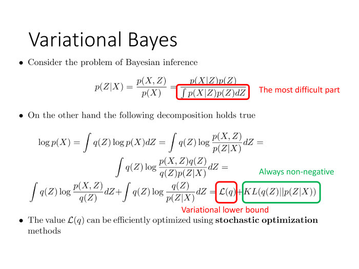
Bayes theorem. According to well-known X, M, we want to say something about Z, which is somehow related to X. We apply the Bayes theorem. Question: what is the most vulnerable place here, what is the hardest fragment? Integral.
In those rare cases when the integral is taken analytically, all is well. It’s another thing if it is not analytically taken - and we imagine that we are talking about high-dimensional data, and here the integral in space with dimensions not 1 or 2, but tens and hundreds of thousands.
On the other hand, let's write a chain. We start: ∫ p (X | Z) p (Z) dZ. Since log P (X) dZ does not depend, it is just an integral over all Z, equal to 1.
The second action. They expressed p (X), transferred to the left by this formula, p (Z | X) in the denominator, recorded under the integral.
Now we have the numerator and denominator depend on Z, although their quotient gives p (X), that is, it does not depend on Z. Identity.
Then multiplied what stands under log, multiplied by 1 and divided by q (Z).
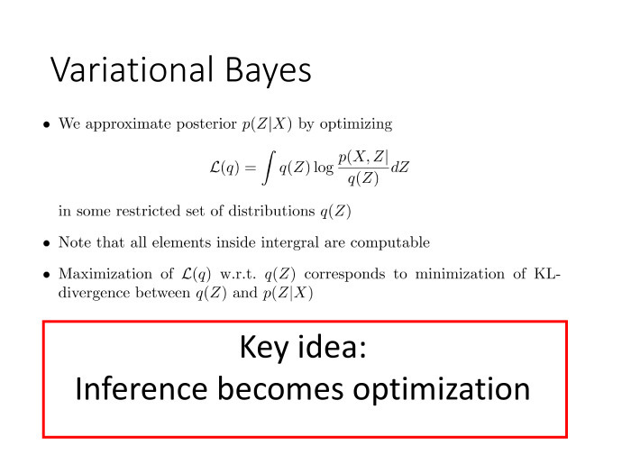
And the last - broke the integral into two parts. Here we see: the second part is the Kullback-Leibler divergence, well-known in probability theory, a non-negative and zero value if and only if these two distributions coincide with each other. In a sense, this is analogous to the distance between distributions. And I remind you that our task is to estimate p (Z | X), at least approximately, to perform Bayesian inference.
We cannot calculate this value; here p (Z | X) appears. But we can perfectly calculate the first term. Each of the terms depends on q (Z), but their sum does not depend on q (Z), because it is equal to log p (X). An idea arises: let us be the first item to be maximized in q (Z), in distribution.
This means that, by maximizing the first term, we minimize the second — which shows the degree of approximation of q (Z) to the true a posteriori distribution. , , : , , .
.
. — .
, ? ? .
.
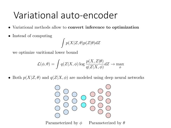
— . X tr , Z , θ. , , L, θ — θ. L Q(Z) θ. θ , Q(Z) Z.
, . , , , . , , - .
, . , Z Q(Z). , . , .
, . , , , — , , .
. — . : . , , , . .
, , , - . , μ σ — . . , Z i μ σ, X i . θ. . , , .
, : , , . , . L, Q(Z), φ, . , , . , , — , .
. φ. , Z, X. — , X Z.
, . , .
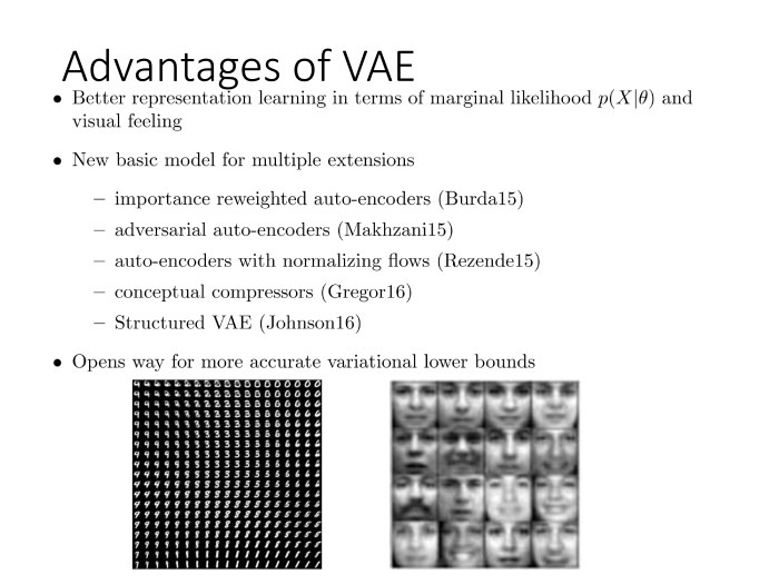
, . , . , , , . representations.
log , , . , — , , , , — . — . - , , , , . . , , , , . .
, . — drop out. , , . , . , . . drop out , , , , .
, , attention maps, , . . , — L(Q|θ).
On this finish. , . , . , NIPS , , — .
, , , . — . Thank.
Under the cut - decoding and part of the slide.
Time a little, I will ride on tops. Those interested can watch the slides - there is a stricter conclusion and many beautiful and different formulas. Let's hope that will not be very boring.
What I will talk about. I will try to give a brief description of Bayesian methods, the Bayesian approach as a probability theory, as a machine learning problem. This approach was quite popular in the 90s and zero years - before the deep revolution started, caused by the triumphal procession of deep neural networks. For some time it seemed: why all these Bayes methods are needed, we have neural networks and so work fine. But as often happens, at some point it turned out that the advantages of the neural network and Bayesian approaches can be combined. First of all, due to the fact that the techniques of variational Bayes output appeared, and these models do not contradict each other, but on the contrary, they perfectly complement each other, reinforcing each other.
')
In a sense, I perceive it as a direction for the further development of modern machine learning and deep learning. It is important to understand that neural networks are not a panacea. They are just an important step in the right direction, but not the last step. I will try to talk about the next possible step in machine learning theory. And the next speaker, Sergey Bartunov, will try to engage in the deconstruction of the myth and in some sense continue the idea that in-depth training is not a panacea. But Sergey will approach this somewhat from the other side, will provide some more global view.
So what is the Bayesian approach? The whole approach is based on a single formula or theorem. Bayes theorem is given in mathematical and conceptual forms.
Key idea Suppose there is some unknown quantity that we would like to evaluate for some of its indirect manifestations. In this case, the unknown quantity is θ, and its indirect manifestation is y. Then you can use the Bayes theorem, which allows our initial ignorance or knowledge of an unknown quantity, a priori knowledge, to transform into a posteriori after observing some indirect characteristics, somehow indirectly characterizing the unknown quantity θ.
The key feature of the formula is that we input an a priori distribution that encodes our ignorance or our uncertainty about an unknown value, and that the output is also a distribution. This is a very important point. Not a point estimate, but a certain entity of the same format that was at the entrance. Due to this, it becomes possible, for example, to use the Bayesian inference, a posteriori distribution, as a priori in some new probabilistic model and, thus, to characterize a new unknown value from different sides by analyzing its various indirect manifestations. This is the first advantage due to which it is possible to obtain the extensibility property - or compositionability - of different probabilistic models, when we can build more complex ones from simple models.
The second interesting property. The simplest rule for summing the product of probabilities is: if we have a probabilistic model — in other words, a joint probability distribution for all variables arising in our problem — then, at least in theory, we can always construct any probabilistic forecast, predict the variable of interest U, knowing some observable variables O. In this case, there is a variable L, which we do not know and does not interest us. According to this formula, they are perfectly excluded from consideration.
For any combination of these three groups of variables, we can always construct such a conditional distribution, which will indicate how our ideas about the quantities U of interest to us have changed, if we have observed the O values supposedly related to U.
In fact, the widespread use of Bayes formulas gave birth to a second alternative approach to probability theory. There is a classic approach - often called frequency, phreakventist in the West - and there is an alternative Bayesian approach. Here is a brief table that I give in all my lectures and which shows the differences between the approaches. Naturally, they do not contradict each other. They rather complement each other. On this label you can see what they have in common and what are the differences.
The key difference is what is meant by a random variable. In frequency terms, we understand by a random variable a quantity, the value of which we cannot predict without appreciating any statistical patterns. Something with objective uncertainty is needed, while in the Bayesian approach the random variable is interpreted simply as a deterministic process. It can be fully predicted. Just in this deterministic process, we do not know part of the factors that influence the outcome. Since we do not know them, we cannot predict the outcome of the deterministic process. So, for us, this outcome looks like a random variable.
The simplest example is a coin flip. This is a classic random value, but we understand that the coin obeys the laws of classical mechanics and, in fact, knowing all the initial conditions — force, acceleration, coefficient of resistance of the medium, etc. — we could say for sure will fall: an eagle or tails.
If you think about it, the overwhelming majority of the quantities that we used to think of as random are actually random in the Bayesian sense. These are some deterministic processes, we just do not know part of the factors of these processes.
Since one may not know some factors, and the other - others, the concept of subjective uncertainty or subjective ignorance arises.
The rest is the direct difference between this interpretation. All values in the Bayesian approach can be interpreted as random. The apparatus of probability theory is applied to the distribution parameters of a random variable. In other words, the fact that in the classical approach is meaningless, in the Bayesian approach makes sense. The method of the statistical method, instead of the maximum likelihood method - Bayes theorem. Estimates are not point-like, but a kind of posterior distribution, allowing us to combine different probabilistic models. And unlike the frequency approach - theoretically justified for large n, and some prove, for example, when n tends to infinity - the Bayesian approach is true for any sample size, even if n = 0. Just in this case, the a posteriori distribution will coincide with the prior .
Simple illustration. A famous parable about blind wise men and an elephant, showing how a model can be hooked.
Let's imagine: given several blind sages and one elephant. The task is to estimate the mass of this elephant. Wise men know that they will now feel a certain animal. What exactly - do not know, but they have to evaluate the mass.
They all start by coding their ideas about the possible mass of an animal in the form of an a priori distribution, since now the distribution density can determine a simple measure of our ignorance about something. To encode this knowledge, we can simply use the apparatus of probability theory.
As far as sages are concerned, they know the characteristic masses of animals on planet Earth. Therefore, they get about this prior distribution.
The first sage comes up, feels the tail and concludes that, apparently, there is something snake-like or the tail of a large animal in front of him. Hence, in the process of his Bayesian inference, by combining the results of his representations, which can be expressed in the form of a probability partition p1, he obtains the posterior distribution p (θ) under the condition x = 1.
Then comes another sage who can not feel, but say, sniff. There is a completely different model. X2 is a value from a completely different domain, indirectly characterizing the mass of the animal. In the process of his Bayesian inference, he uses, as an a priori distribution, not the initial distribution from which everyone started, but the result of the output of the previous sage. Thus, we can combine two completely different dimensions, two sources of information, in one elegant probabilistic model.
And so, having done a series of measurements, we end up with a fairly sharp a posteriori distribution, an almost accurate estimate. We can already say with high accuracy what weight the animal had. This is an illustration of the third property - to extendibility, that is, the ability of the model to expand and hook all the time.
Another advantage of the Bayesian approach, already applied to machine learning, is regularization. By taking into account a priori preferences, we prevent the excessive adjustment of our parameters during the machine learning procedure and are thus able to cope with the effect of retraining. Some time ago, when the algorithms began to train on huge amounts of data, it was thought that the problem of retraining was removed from the agenda. But it was all about the fact that people were psychologically afraid to switch to giant-sized neural networks. Everyone started with small neural networks, and they, with giant training samples, did not really retrain. But as psychological fear disappeared, people began to use larger networks.
Two things have become obvious. For a start, the larger the network, the better it is in principle. Large networks work better than small ones. But large networks are starting to retrain. If we have a number of parameters - 100 million, then 1 billion objects are not a very large training sample, and we need to regularize the procedure of such machine learning.
The Bayesian approach provides an excellent opportunity to do this by introducing an a priori distribution on those parameters, on those neural network weights that are configured during the training procedure.
In particular, it turned out that such a popular heuristic regularization technique, such as drop out, is a special case, a rough approximation for Bayesian regularization. In fact, this is an attempt to make a Bayesian conclusion.
Finally, the third advantage is the ability to build a model with latent variables. About her more.
We have a motivating example - the main component method. The method is very simple - linear reduction of the dimension. We take a sample in space with a high dimension, build a covariance matrix, project it onto the main axis with the corresponding largest value. Here is what is geometrically shown here. And reduced the dimension of the space from 2 to 1, while maintaining the maximum dispersion contained in the sample.
The method is simple, allows the solution in an explicit form. But you can alternatively formulate differently, in terms of a probabilistic model.
Imagine that our data is arranged as follows: for each object there is its hidden representation in a space of small dimension. Here, it is labeled z. And we observe a linear function of this hidden representation in space with a higher dimension. We took a linear function and additionally added normal noise. Thus, we obtained x, high-dimensional data, according to which it is highly desirable for us to restore their low-dimensional representation.
Mathematically, it looks like this. We set a probabilistic model, which is the joint probability distribution for observable and hidden components, on x and z. The model is quite simple, the sample is characterized by the product of objects. The observable component of each object is determined by the hidden component; we are talking about a priori distribution on the hidden component. Both are normal distributions. We assume that in a small space the data is distributed a priori normally, and we observe a linear function of this data, which is noisy with normal noise.
We are given a sample, which is a high-dimensional representation. We know x, we do not know z, and our task is to find the parameter θ. θ is the V, σ² matrix and that's it.
This problem can be formulated in Bayesian language as a learning task with latent variables. To apply the usual maximum likelihood method, there is not enough knowledge of increasing z. It turns out that for this technique there is a standard approach based on the EM algorithm and various modifications. You can run an iterative process. The EM-step contains formulas describing what we are doing. It can theoretically be shown that the process is monotonous and is guaranteed to converge to a local extremum, but still.
The question arises: why do we need to use the iterative process, when we know that the problem is solved explicitly?
The answer is simple. To begin with - algorithmic complexity. The complexity of the analytical solution is O (nD²), while the complexity of one iteration of the EM algorithm is O (nDd).
If we mentally imagine that we are projecting a space of 1 million in space with a dimension of 10, and the EM algorithm converges iterations over one hundred, then our iterative scheme will work 1000 times faster than an explicit solution.
In addition, an important advantage: now we can expand our basic model, the method of principal components, in various ways, depending on the specifics of a specific task. For example, we can introduce the concept of a mixture of methods of principal components, and say that our data does not live in one space, a linear subspace of a lower dimension, but in several. And we do not know from which subspace each particular object came.
There is a mixture of main component methods. Formally, the model is written as follows. Just entered the additional nomenclature of hidden discrete variables t. And again, the EM-algorithm allows us to find a solution to the problem using almost the same formulas, although the original method of the main components did not allow us to make any modifications.
Another one is the ability to work in situations where, say, for our sample, part of the components of x are unknown, the data is missing. It happens? Pretty often. Somewhat more exotic situation - when we know the hidden views of parts of objects, low-dimensional view, in whole or in part. But again, this situation is possible.
The original model of the principal component method is incapable of taking into account either one or the other, while the probabilistic model formulated in Bayesian language takes both of them elementary - by a simple modification of the EM algorithm. We simply change the nomenclature of observable hidden variables.
Thus, we can solve data processing tasks, when some arbitrary fragments of this data may be absent, not like in standard machine learning, when a nomenclature of observable and seemingly hidden target variables is allocated, they can in no way intermix. This is where additional flexibility arises.
Finally, until recently, it was believed that a significant limitation of Bayesian methods is that, with their high computational complexity, they are applicable to small data samples and are not transferred to big data. The results of the last few years show that this is not the case. Humanity has finally learned to provide the scalability of Bayesian methods. And people immediately began to cross Bayesian methods with deep neural networks.
I will say a few words on how to scale the Bayesian method, there is still time to benefit.
Bayes theorem. According to well-known X, M, we want to say something about Z, which is somehow related to X. We apply the Bayes theorem. Question: what is the most vulnerable place here, what is the hardest fragment? Integral.
In those rare cases when the integral is taken analytically, all is well. It’s another thing if it is not analytically taken - and we imagine that we are talking about high-dimensional data, and here the integral in space with dimensions not 1 or 2, but tens and hundreds of thousands.
On the other hand, let's write a chain. We start: ∫ p (X | Z) p (Z) dZ. Since log P (X) dZ does not depend, it is just an integral over all Z, equal to 1.
The second action. They expressed p (X), transferred to the left by this formula, p (Z | X) in the denominator, recorded under the integral.
Now we have the numerator and denominator depend on Z, although their quotient gives p (X), that is, it does not depend on Z. Identity.
Then multiplied what stands under log, multiplied by 1 and divided by q (Z).
And the last - broke the integral into two parts. Here we see: the second part is the Kullback-Leibler divergence, well-known in probability theory, a non-negative and zero value if and only if these two distributions coincide with each other. In a sense, this is analogous to the distance between distributions. And I remind you that our task is to estimate p (Z | X), at least approximately, to perform Bayesian inference.
We cannot calculate this value; here p (Z | X) appears. But we can perfectly calculate the first term. Each of the terms depends on q (Z), but their sum does not depend on q (Z), because it is equal to log p (X). An idea arises: let us be the first item to be maximized in q (Z), in distribution.
This means that, by maximizing the first term, we minimize the second — which shows the degree of approximation of q (Z) to the true a posteriori distribution. , , : , , .
.
. — .
, ? ? .
.
— . X tr , Z , θ. , , L, θ — θ. L Q(Z) θ. θ , Q(Z) Z.
, . , , , . , , - .
, . , Z Q(Z). , . , .
, . , , , — , , .
. — . : . , , , . .
, , , - . , μ σ — . . , Z i μ σ, X i . θ. . , , .
, : , , . , . L, Q(Z), φ, . , , . , , — , .
. φ. , Z, X. — , X Z.
, . , .
, . , . , , , . representations.
log , , . , — , , , , — . — . - , , , , . . , , , , . .
, . — drop out. , , . , . , . . drop out , , , , .
, , attention maps, , . . , — L(Q|θ).
On this finish. , . , . , NIPS , , — .
, , , . — . Thank.
Source: https://habr.com/ru/post/321434/
All Articles