How to evaluate the quality of the A / B testing system

For more than half a year, the company has used a unified system for conducting A / B experiments. One of the most important parts of this system is the quality control procedure, which helps us understand how much we can trust the results of A / B tests. In this article, we describe in detail the principle of the quality control procedure for those readers who want to test their A / B testing system. Therefore, the article has many technical details.

A few words about A / B testing

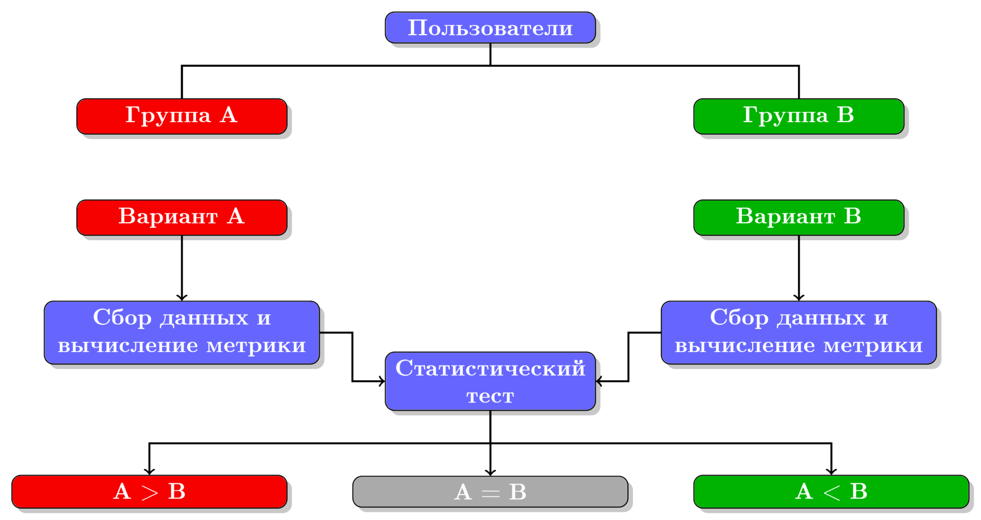
Figure 1. Scheme of the A / B testing process.

In general, the A / B testing process can be divided into the following steps (shown in the figure):
')

Distribution of users in two groups A and B.
Presentation of two different options to two user groups.
Data collection and calculation of metric values for each group.
Comparison of metric values in both groups using a statistical test and deciding which of the two options won.

In principle, using the A / B tests, we can compare any two options, but for definiteness we will assume that group A is shown the current version working in production, and group B is an experimental version. Thus, group A is the control group, and group B is the experimental one. If users in group B are shown the same option as in group A (that is, there is no difference between options A and B), then this test is called the A / A test.

If one of the options won in the A / B test, then they say that the test has become painted over.

History of A / B testing in a company

A / B testing at HeadHunter began, one might say, spontaneously: development teams arbitrarily divided the audience into groups and conducted experiments. At the same time, there was no common pool of verified metrics - each team calculated its own metrics from user activity logs. There was no common system for determining the winner either: if one option was far superior to the other, then he was declared the winner; if the difference between the two options was small, then statistical methods were used to determine the winner. The worst thing was that different teams could conduct experiments on the same group of users, thereby influencing each other’s results. It became clear that we need a unified system for conducting A / B tests.

Such a system was created and launched in July 2016. With this system, the company has already conducted 77 experiments. The number of A / B experiments by month is shown in Figure 2.

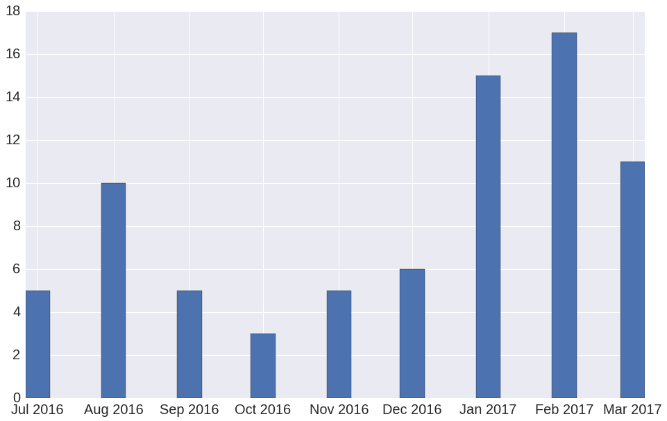
Figure 2. The number of A / B experiments by month since the launch of the A / B testing system. The number of experiments for March 2017 is incomplete, because at the time of publication this month is not over yet.

When creating the A / B testing system, we paid the most attention to the statistical test. First of all, we were interested in the answer to the following question:

How to make sure that the statistical test does not deceive us and we can trust its results?

The question is not idle, because the harm from the incorrect results of the stat. test may be even more than the lack of results.

Why we may have reasons not to trust the stat. test? The fact is that the statistical test involves a probabilistic interpretation of the measured values. For example, we consider that each user has a “probability” to perform some kind of successful action (registration, purchase of goods, likes, etc.) can be successful actions. At the same time, we consider the actions of different users independent. But initially we do not know how well the actions of users correspond to the probabilistic model of stat. test.

In order to assess the quality of the A / B testing system, we conducted a large number of A / A tests and measured the percentage of stained tests, that is, the percentage of cases in which a stat. the test was wrong in asserting the statistically significant superiority of one variant over the other. The benefits of A / A tests can be found, for example, here . Measured error rate stat. the test was compared with a given theoretical value: if they are approximately the same, then everything is fine; if the measured error rate is much less or much more than the theoretical, then the results of such a stat. dough unreliable.

To tell more about the method of assessing the quality of the A / B testing system, you must first talk about the level of significance and about other concepts that arise when testing statistical hypotheses . Readers familiar with this topic may skip the next paragraph and go to the A / B Testing System Quality Assessment paragraph.

Statistical test, confidence intervals and significance level

Let's start with a simple example. Suppose we have only 6 users and we have divided them into 2 groups of 3 people, conducted the A / B test, calculated the value of the metric for each individual user and obtained the following tables:

Table 1. Group A, Mean Metric $\ widehat {\ mu} _ {A} = \ dfrac {1} {3}$
User	Metric value
A. Antonov	one
P. Petrov	0
S. Sergeev	0

Table 2. Group B, Mean Metric $\ widehat {\ mu} _ {B} = \ dfrac {2} {3}$
User	Metric value
B. Bystrov	0
V. Volnov	one
U. Umnov	one

The average value of a metric in group A is equal to

$\ widehat {\ mu} _ {A} = \ dfrac {1} {3}$ in group B -

$\ widehat {\ mu} _ {B} = \ dfrac {2} {3}$ and the average difference between the two groups is

$\ widehat {\ mu} _ {\ Delta} = \ widehat {\ mu} _ {B} - \ widehat {\ mu} _ {A} = \ dfrac {1} {3}$ . If we confine ourselves to the average values, it turns out that the variant shown for group B won (since the difference

$\ widehat {\ mu} _ {\ Delta}$ Above zero). But in each group there are only 3 values - it means that we estimated the true value of the difference by 6 numbers, that is, with a large error. Therefore, the result can be random and can mean nothing.

That is, besides the difference between the average values of the metrics in the two groups, we would also like to evaluate the confidence interval for the true value of the difference

$\ mu _ {\ Delta}$ , that is, the interval in which, “most likely,” is the true value. The phrase "most likely" has an intuitive meaning. To formalize it, the concept of significance level is used.

$\ alpha$ . The level of significance is related to the confidence interval and reflects the degree of our confidence that the true value is within this confidence interval. The lower the level of significance, the more confident we are.

Imagine what the level of significance means, you can. If we repeat the A / A test many times, the percentage of cases in which the A / A test gets stained will be approximately equal to

$\ alpha$ . That is, in

$\ alpha \%$ cases, we reject the equality of options hypothesis, although both options are really equal (in other words,

$\ alpha \%$ cases we make a mistake of the first kind ). We chose significance to be equal to

$\ alpha = 5 \%$ .

Actually, the statistical test is just engaged in estimating the confidence interval for the difference

$\ mu _ {\ Delta}$ for a given level of significance. If the confidence interval is known, then the procedure for determining the winner is simple:

If both limits of the confidence interval are greater than 0, then B has won.
If 0 is inside the interval, then a draw means that none of the options won.
If both borders are less than 0, then won option A.

For example, suppose we were somehow able to find out that for the level of significance

$\ alpha = 5 \%$ the confidence interval for the difference in our example is

$\ widehat {\ mu} _ {\ Delta} \ pm \ dfrac {1} {2} \ rightarrow \ dfrac {1} {3} \ pm \ dfrac {1} {2} \ rightarrow \ left [- \ dfrac {1} {6}, \ dfrac {5} {6} \ right]$ . That is, the true value of the difference

$\ mu _ {\ Delta}$ most likely lies inside the interval

$\ left [- \ dfrac {1} {6}, \ dfrac {5} {6} \ right]$ . Zero belongs to this interval - it means that we have no reason to assume that one of the options is better than the other (in fact, one of the options may be better than the other, we simply do not have enough data to assert this with a significance level of 5%) .

It remains for us to understand how the statistical test from the significance level and experimental data estimates the confidence intervals for the difference in metric values between groups A and B.

Determination of confidence intervals

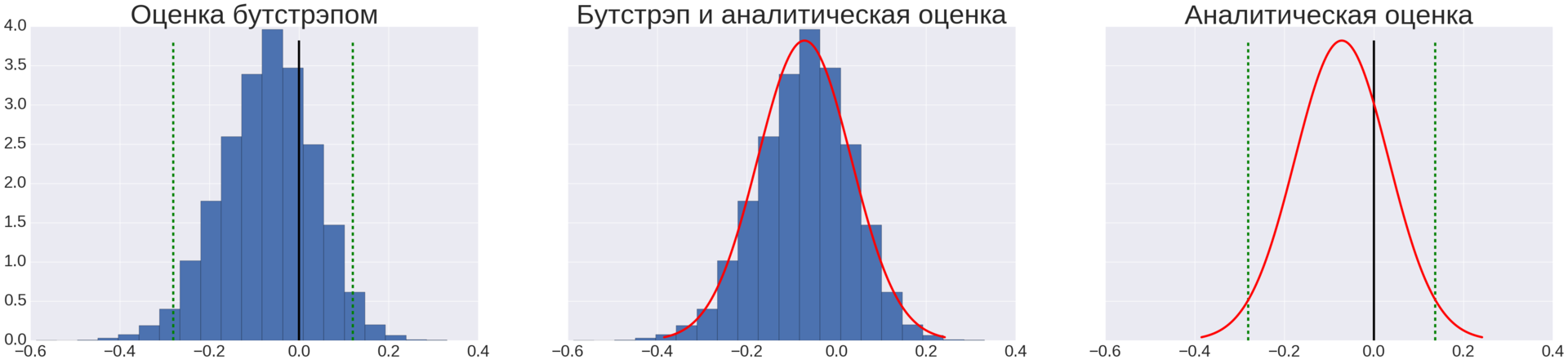
Figure 3. Estimation of the confidence intervals for the difference

$\ mu _ {\ Delta}$ using bootstrap (left graph, 10 000 iterations of bootstrap) and analytically (right graph). The green line shows the boundaries of the confidence interval, the black line - the position of zero. On the average chart, both methods are combined for comparison.

To determine the confidence intervals, we used two methods, shown in Figure 3:

Analytically.
With bootstrap.

Analytical estimation of confidence intervals

In the analytical approach, we rely on the statement of the central limit theorem (CLT) and expect that the difference in the mean values of metrics in the two groups will have a normal distribution, with parameters

$\ mu _ {\ Delta}$ and

$\ sigma _ {\ Delta}$ . Exact values

$\ mu _ {\ Delta}$ and

$\ sigma _ {\ Delta}$ we do not know, but we can calculate the approximate estimates

$\ widehat {\ mu} _ {\ Delta}$ and

$\ widehat {\ sigma} _ {\ Delta}$ :

$\ begin {eqnarray *} \ widehat {\ mu} _ {\ Delta} & = & \ widehat {\ mu} _B - \ widehat {\ mu} _A \\ \ widehat {\ sigma} _ {\ Delta} & = & \ sqrt {\ widehat {\ sigma} _A ^ 2 + \ widehat {\ sigma} _B ^ 2} \ end {eqnarray *}$

Where are mean values (

$\ widehat {\ mu} _A, \ widehat {\ mu} _B$ ) and mean value variances (

$\ widehat {\ sigma} _A, \ widehat {\ sigma} _B$ ) are calculated

according to standard formulas.

$\ begin {eqnarray *} \ widehat {\ mu} _A & = & \ dfrac {1} {N_A} \ sum_ {i = 1} ^ {N_A} x_i \\ \ widehat {\ mu} _B & = & \ dfrac {1} {N_B} \ sum_ {j = 1} ^ {N_B} x_j \\ \ widehat {\ sigma} _A ^ 2 & = & \ dfrac {1} {N_A (N_A - 1)} \ sum_ {i = 1} ^ {N_A} (x_i - \ widehat {\ mu} _A) ^ 2 \\ \ widehat {\ sigma} _B ^ 2 & = & \ dfrac {1} {N_B (N_B - 1)} \ sum_ { j = 1} ^ {N_B} (x_j - \ widehat {\ mu} _B) ^ 2 \ end {eqnarray *}$

Knowing the parameters of the normal distribution and the level of significance, we can calculate the confidence intervals. The formulas for calculating confidence intervals are not given, but the idea is shown in Figure 3 on the right graph.

One of the drawbacks of this approach is the fact that random variables in the CLT are assumed to be independent. In reality, this assumption is often violated, in particular, due to the fact that the actions of one user are dependent. For example, an Amazon user who bought one book is likely to buy another one. It will be a mistake to consider two purchases of one user as independent random variables, because as a result we can get too optimistic estimates for the confidence interval. And this means that in reality, the percentage of falsely overflowed A / A tests can be many times larger than the specified value. This is what we observed in practice. Therefore, we tried another method for estimating confidence intervals, namely bootstrap.

Estimation of confidence intervals using bootstrap

Bootstrap is one of the methods of non-parametric estimation of confidence intervals, in which no assumptions about the independence of random variables are made. Using bootstrap to estimate confidence intervals comes down to the following procedure:

To repeat N textrmbootstrap time:
- using bootstrap, select random subsamples of values from groups A and B;
- calculate the difference of averages $\ widehat {\ mu} _ {\ Delta_i}$ in these subsamples;
Sort ascending values obtained at each iteration
Using an ordered array $\ left [\ widehat {\ mu} _ {\ Delta_1}, \ widehat {\ mu} _ {\ Delta_2}, ~ \ dots ~ \ widehat {\ mu} _ {\ Delta_ {N _ {\ textrm {bootstrap} }}} \ right]$ determine the confidence interval so that $\ sim (1- \ alpha) \ cdot N _ {\ textrm {bootstrap}}$ points lay inside the interval. That is, the left border of the interval will be the number with the index
$\ dfrac {\ alpha} {2} \ cdot N _ {\ textrm {bootstrap}}$ and the right border is a number with an index $(1 - \ dfrac {\ alpha} {2}) \ cdot N _ {\ textrm {bootstrap}}$ in an ordered array.

Figure 3 on the left graph shows a histogram for the array of difference values obtained after 10,000 bootstrap iterations and confidence intervals calculated by the procedure described here.

A / B Testing System Quality Assessment

So, we have broken all users into

$N_ \ textrm {groups}$ groups, prepared a statistical test and chose the metric that we want to improve. Now we are ready to evaluate the quality of the A / B testing system. In HeadHunter we were interested in how often the stat. the test will make a mistake of the first kind, that is, what percentage of A / A tests will stain (we denote this value

$\ alpha ^ \ textrm {real}$ ) at a fixed level of significance

$\ alpha$ .

Calculate

$\ alpha ^ \ textrm {real}$ we can do a lot of A / A tests. As a result, we can get three options:

If a $\ alpha ^ \ textrm {real} \ ll \ alpha$ then either stat. test or selected metric is too conservative. That is, A / B tests have low sensitivity (“resistant tin soldier”). And this is bad, because in the course of operating such an A / B testing system, we will often reject changes that really improved, because we did not feel any improvement (i.e., we will often make the second error kind of ).
If a $\ alpha ^ \ textrm {real} \ gg \ alpha$ then either stat. test, or the selected metric is too sensitive ("Princess and the Pea"). This is also bad, because during operation we will often accept changes that in reality did not affect anything (that is, we will often make a mistake of the first kind ).
Finally if $\ alpha ^ \ textrm {real} \ approx \ alpha$ means stat. test together with the selected metric show good quality and such a system can be used for A / B testing.


(a) enumerate all possible pairs	(b) Randomly split into disjoint pairs.
Figure 4. Two options for partitioning 4 user groups ( $G_1$ , $G_2$ , $G_3$ , $G_4$ a) on pairs.

So, we need to do a lot of A / A tests in order to better assess the percentage of stat errors. test

$\ alpha ^ \ textrm {real}$ . For this we need a large number of pairs of user groups. But where can we get a large number of pairs if all users are divided into a small number of groups (we divided users into 64 groups). The first thing that comes to mind is to make all sorts of pairs of groups. If the number of user groups we have is

$N_ \ textrm {groups}$ then we can make one of them

$\ dfrac {N_ \ textrm {groups} (N_ \ textrm {groups} - 1)} {2}$ different pairs (the pairing scheme for 4 groups is shown in Figure 4 (a)).

However, this approach has a serious drawback , namely: we get a large number of dependent pairs. For example, if in one group the average value of the metric is very small, then most A / A tests for pairs containing this group will stain. Therefore, we stopped at the approach shown in Figure 4 (b), in which all groups are divided into disjoint pairs. That is, the number of pairs is equal to

$\ dfrac {N_ \ textrm {groups}} {2}$ . The steam turned out to be much smaller than in the first method, but now they are all independent.

The results of applying the A / A test to 64 groups of users, which were divided into 32 independent pairs, are shown in Figure 5. From this figure, it can be seen that out of 32 pairs only 2 were colored, i.e.

$\ alpha ^ \ textrm {real} = 2/32 \ cdot 100 \% \ approx 6 \%$ .

Figure 5. A / A test results for 64 user groups randomly split into 32 pairs. Confidence intervals were calculated using bootstrap, the significance level was 5%.

Value histograms

$\ left [\ widehat {\ mu} _ {\ Delta_1}, \ widehat {\ mu} _ {\ Delta_2}, ~ \ dots ~ \ widehat {\ mu} _ {\ Delta_ {N _ {\ textrm {bootstrap} }}} \ right]$ received by bootstrap are shown in blue for non-tinted couples, yellow for stained ones; Gaussian distribution with analytically calculated parameters is shown in red. The black line indicates the zero position.

In principle, this could be stopped. We have a way to calculate the real percentage of stat errors. test. But in this way we were confused by a small number of A / A tests. It seems that 32 A / A test is not enough for reliable measurement of

$\ alpha ^ \ textrm {real}$ . So, it remains for us to answer the following question:

If the number of pairs is small, how can we reliably measure

$\ alpha ^ \ textrm {real}$ ?

We used this solution: let's randomly redistribute users into groups many times. And after each redistribution we will be able to measure the percentage of errors

$\ alpha ^ \ textrm {real} _ {i}$ . The average of all measured values will give an estimate of

$\ alpha ^ \ textrm {real}$ .

As a result, we obtained the following procedure for assessing the quality of the A / B testing system:

To repeat N textrmiterations time:
- Randomly distribute all users by $N_ \ textrm {groups}$ groups;
- Accidentally break $N_ \ textrm {groups}$ groups on $\ dfrac {N_ \ textrm {groups}} {2}$ steam;
- For all pairs, perform an A / A test and calculate the percentage of overgrown steam. $\ alpha ^ \ textrm {real} _i$ on this $i$ iteration
calculate $\ alpha ^ {\ textrm {real}}$ as average for all iterations:
$$ display $$ \ begin {equation *} \ alpha ^ {\ textrm {real}} = \ dfrac {1} {N_ \ textrm {iterations}} \ sum_ {i = 1} ^ {N_ \ textrm {iterations} } \ alpha ^ \ textrm {real} _i \ end {equation *} $$ display $$

If in the procedure for assessing the quality of the A / B testing system, we fix a stat. test (for example, we will always use bootstrap) and believe that the stat itself. If the test is infallible (or irreplaceable), then we will have a system for assessing the quality of metrics .

An example of assessing the quality of one of the metrics is shown in Figure 6. From this graph it can be seen that the average percentage of stat errors. test (i.e. value

$\ alpha ^ \ textrm {real}$ ) almost perfectly coincides with the specified value

$\ alpha = 5 \, \%$ . It is worth noting that such a good coincidence we have seen infrequently. We consider it a good coincidence if

$3 \, \% \ leq \ alpha ^ \ textrm {real} \ leq 8 \, \%$ .

Figure 6. The result of the quality assessment for the metrics of successful user actions. Blue shows a histogram for an array of numbers

$\ left [\ alpha ^ \ textrm {real} _1, \ alpha ^ \ textrm {real} _2 ~ \ dots ~ \ alpha ^ \ textrm {real} _ {N_ \ textrm {iterations}} \ right]$ , green - average value of the array, black - the specified level of significance for bootstrap (the number of bootstrap iterations is 10,000). The number of user group pairs is 32. The number of iterations of the quality assessment procedure

$N_ \ textrm {iterations} = 1000$ .

Metrics Quality Assessment Results


(a)	(b)	(at)
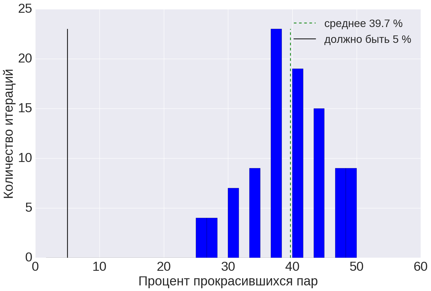
Figure 7. Quality assessment results for the metrics of the success of the search sessions: (a) for the initial metric and bootstrap by values, (b) for the initial metrics and bootstrap for users, (c) for modified metrics and bootstrap for values.

When we applied the quality assessment procedure to the metrics of the success of the search sessions, we got the result as in Figure 7 (a). Stat. The test in theory should be wrong in 5% of cases, but in reality it is wrong in 40% of cases! That is, if we use this metric, then 40% of the A / B tests will be painted over, even if option A is no different from option B.

This metric turned out to be a “princess on a pea”. However, we still wanted to use this metric, as its value has a simple interpretation. Therefore, we began to understand what could be the problem and how to deal with it.

We assumed that the problem may be due to the fact that several values that are dependent on the metric fall from a single user. An example of a situation where two numbers fall into a metric from a single user (Ivan Ivanovich) is shown in Table 3.

Table 3. An example of several values in the metric from one user
User	Metric value
Ivan Ivanovich	0
Ivan Nikiforovich	0
Anton Prokofievich	one
Ivan Ivanovich	one

We can weaken the effect of dependence of the values of one user either by modifying the stat. test or change the metric. We tried both of these options.

Modification of stat. test

Since the values from one user are dependent, we performed the bootstrap not by values, but by users: if the user is included in the bootstrap sample, then all his values are used; if not, none of its values are used. The use of such a scheme led to a significant improvement (Figure 7 (b)) - the real percentage of stat errors. test on 100 iterations was equal

$\ alpha ^ {\ textrm {real}} = 4.8 \%$ which is very close to the theoretical value

$\ alpha = 5.0 \%$ .

Metric Modification

If we are hampered by the fact that several dependent values fall into the metric from one user, then we can first average all the values within the user so that only one number falls into the metric from each user. For example, Table 3, after averaging the values within each user, will go to the following table:

Table 4. Example of aggregation of values within each user
User	Metric value
Ivan Ivanovich	0.5
Ivan Nikiforovich	0
Anton Prokofievich	one

The results of assessing the quality of the metric after this modification are shown in Figure 7 (c). The percentage of cases in which stat. the test was wrong, turned out to be almost 2 times lower than the theoretical value

$\ alpha = 5.0 \%$ . That is, for this metric

$\ alpha ^ \ textrm {real}$ and

$\ alpha$ imperfectly coincide, but this is much better than the initial situation in Figure 7 (a).

Which of the two approaches is better

We used both approaches (modification of a stat. Test and modification of a metric) to assess the quality of different metrics, and for the vast majority of metrics both approaches showed good results. Therefore, you can use the method that is easier to implement.

findings

The main conclusion that we made when assessing the quality of the A / B testing system: it is imperative that the quality of the A / B testing system be assessed). Before you use a new metric, you need to check it. Otherwise, A / B tests run the risk of becoming a form of divination and damage the development process.

In this article, we have tried, as far as possible, to present all the information about the device and the principles of how the quality assessment procedure of the A / B testing system used in the company works. But if you have any questions, feel free to ask them in the comments.

PS

I would like to thank lleo for systematizing the A / B testing process in the company and for carrying out proof-of-concept experiments, the development of which is this work, and p0b0rchy for sharing experience, patient hours of explanation and for generating ideas that formed the basis our experiments.

Source: https://habr.com/ru/post/321386/

All Articles