📜 ⬆️ ⬇️

There are two functions

Hello

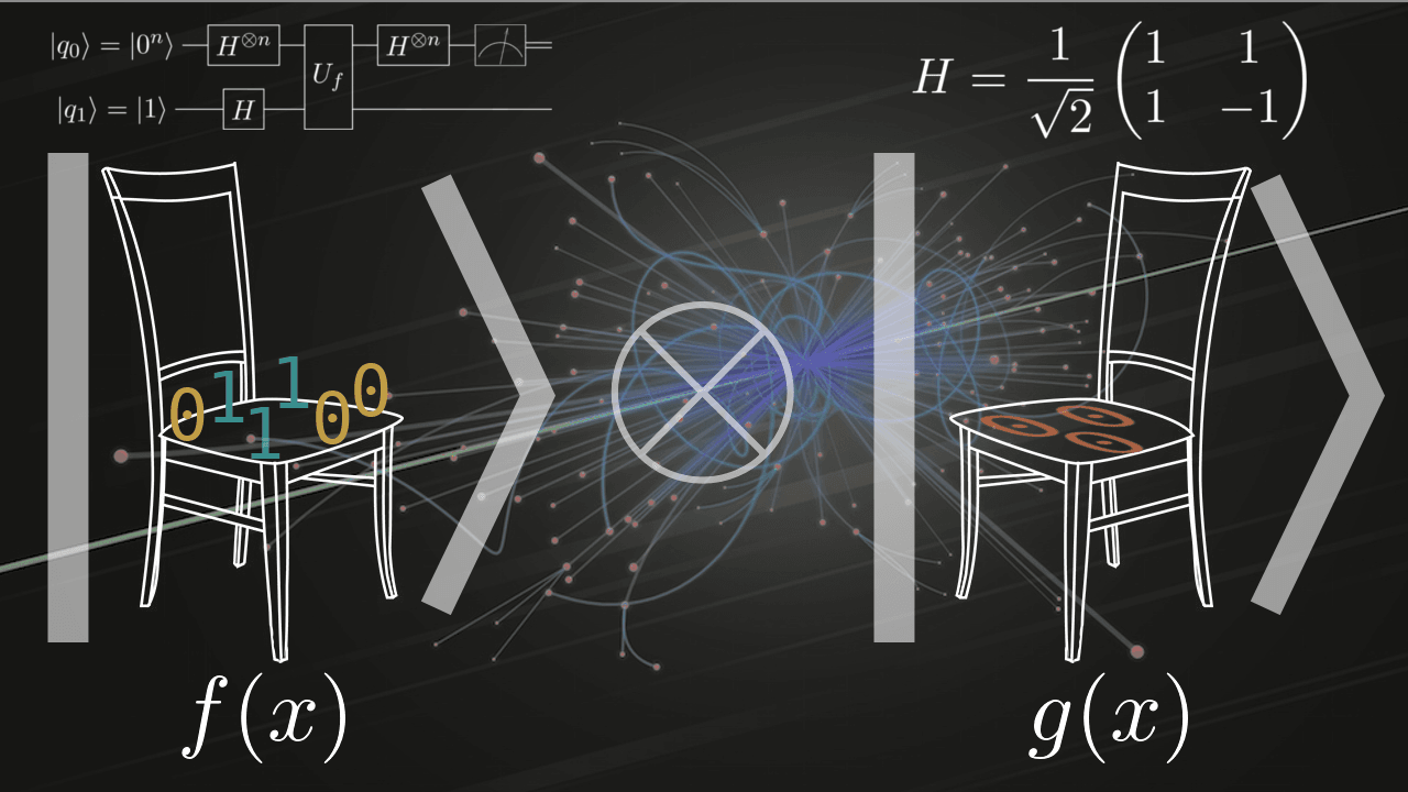
There are two boolean functions. n arguments, one - constant, the other - balanced. Which one will you sit on, which fender? Only functions are unknown, and they can only be called once.

If you do not know how to solve a similar problem, welcome under cat. There I will talk about quantum algorithms and show you how to emulate them in the most popular language - in Python.

I've come to talk with you again


Let's formulate the problem of two functions a little more formally. Let a Boolean function be given. f: \ {0, 1 \} ^ n \ to \ {0, 1 \} and it is known a priori that it is either constant, that is, for any of its arguments, it always returns either 0 or 1, or is balanced, that is, exactly half of its arguments returns 0, and exactly half of it 1. It is required to determine whether the function is constant or balanced. It is considered that the time of the function call is incommensurable more than any other operations, therefore the complexity of the algorithm is determined by the number of function calls.

hard_choice

Example:
')
  1. f (x_1, x_2) = x_1 \ oplus x_2 balanced:
    x_1
    x_2
    f
    000
    0oneone
    one0one
    oneone0

  2. f (x_1, x_2) = x_1 \ vee x_2 \ vee (\ neg x_1 \ wedge \ neg x_2) constant:
    x_1
    x_2
    f
    00one
    0oneone
    one0one
    oneoneone

  3. f (x_1, x_2) = x_1 \ wedge x_2 neither balanced nor constant:
    x_1
    x_2
    f
    000
    0one0
    one00
    oneoneone

The task is, of course, artificial and it is unlikely that someone will ever meet in practice, but it is a classic guide to the brave new world of quantum computing, and I don’t dare break traditions.

Classic deterministic solution


bruteforce

Let's first solve the problem in the classical model of computation. To do this, in the worst case, you need to call the function on 2 ^ {n-1} +1 arguments: exactly half and one more. If all calculated values ​​are the same, then the function is obviously constant. If there are at least two different results, the function is balanced. The complexity of the deterministic algorithm is exponential and is O (2 ^ {n-1} + 1) .

Algorithm in Python:

from itertools import product, starmap, tee def pairwise(xs): a, b = tee(xs) next(b, None) return zip(a, b) def is_constant(f, n): m = 2 ** (n - 1) for i, (x, y) in enumerate(pairwise(starmap(f, product({0, 1}, repeat=n)))): if i > m: break if x != y: return False return True 

Classic probabilistic solution


rasta

But what if, instead of half the arguments, we check a smaller number of them and make a verdict? Exact answer will not be, but with what probability we make a mistake? Let's say we calculated a function on k & lt; 2 ^ {n-1} + 1 arguments. If among the values ​​of the function there are two different, then everything is simple - the function is balanced. Otherwise, we declare it constant with probability p (k) & lt; one . Suppose we are wrong and the function is actually balanced. Calculate the probability of error 1 - p (k) . If we choose the arguments uniformly, then the probability that the two values ​​of the function are equal are the same, 1/2 , and the probability to meet k equal consecutive values ​​equal 1/2 ^ k . In this way:

1 - p (k) = \ frac {1} {2 ^ k},

p (k) = 1 - \ frac {1} {2 ^ k}.

Reverse function:

k (p) = \ log_2 {\ frac {1} {1 - p}}.

With fixed p the complexity of the classical probabilistic algorithm is constant and equal to O (\ log_2 {\ frac {1} {1 - p})}. To be sure of the 99.99% response, you need to call the function only 14 times.

Algorithm in Python:

 import random from itertools import product, starmap, tee def pairwise(xs): a, b = tee(xs) next(b, None) return zip(a, b) def is_constant(f, n, k=14): xs = list(product({0, 1}, repeat=n)) random.shuffle(xs) xs = xs[:k] for x, y in pairwise(starmap(f, xs)): if x != y: return False return True 

And if I tell you that there is a constant deterministic solution with complexity O (1) allowing to call a function only once?

However, before you consider it, you will have to digress ...

Because a vision softly creeping


Myths


Before starting, I would like to discuss a few common myths associated with quantum computing:

  1. Quantum algorithms are hard.

    difficult

    Yes, they are difficult to synthesize, because it requires for this mathematical imagination and insight. They are difficult to implement on real quantum computers: for this you need to know the physics perfectly and stay up late every day in the laboratory at the department. But what exactly does not require any special knowledge and an incredible amount of zeal is their understanding. I argue that everyone can understand quantum algorithms : they rely on extremely simple mathematics, accessible to any freshman. All that is required of you - just a little time to study.

  2. There are already quantum computers on thousands of qubits from D-Wave
    No, these are not real quantum computers.

  3. There is not a single real quantum computer.
    No, there are. In the laboratory, and they have only a few qubits.

  4. Quantum computers will allow to solve problems that were previously unavailable.
    No, the set of problems computable in the classical and quantum models coincide. Quantum computing only reduces the complexity of a small subset of these problems.

  5. On the Crysis quantum computer at max speeds will fly

    wat

    With the exception of a certain subset of problems that the quantum model of computation is capable of speeding up, the rest can be solved only by emulating a classical computer. Which, as you understand, is very slow. Crysis is likely to lag.

  6. A quantum computer is a black box with input and output, looking into which you can ruin everything.

    blackbox

    If you are 12 years old, this analogy will fit. In any other case, it, like all other analogies with boxes, cats, loops and electrons “bound” by threads, so actively promoted in all popular science sources, only confuses, creates the illusion of false understanding and is more harmful than useful. Discard these analogies.

What for?


Why should an applied mathematics (programmer) be able to understand quantum algorithms at the application level? Everything is simple, I am ready to offer you two reasons:

  1. For self-development. Why not?
  2. They are already coming. They are quantum computers. They are already near. You will not have time to blink, as a couple will appear in the server of your company, and in a few more years in the form of a coprocessor in your laptop. And there will be nowhere to run. We'll have to program for them, call quantum coroutines. And without understanding it is difficult to do, agree.

I was sleeping


The most basic component of quantum computing is a quantum system. A quantum system is a physical system, all of whose actions are comparable in magnitude with the Planck constant. This definition and the fact that quantum systems obey the laws of matrix mechanics - all the knowledge that we need from physics. Next - only math.

loldontinterrupt

Like any other physical system, a quantum system can be in a certain state. All possible states of a quantum system form a Hilbert space \ mathcal {H} over the field of complex numbers. I hope the reader is familiar with the concept of complex numbers - their understanding is necessary everywhere in the future. If not, I advise you to meet and come back. The Hilbert space is a complete normed metric linear space with norm \ Vert x \ Vert = \ sqrt {(x, x)} where (x, y) - scalar product. In order from the end:

  1. Linear (vector) space - a set of elements X with the operations of addition of elements introduced on it x + y and multiplications x \ cdot \ lambda on field item K (in our case, the field of complex numbers). These operations must be closed (the result must belong to the set X ) and must be fulfilled 8 axioms. View a full list of them, as well as get acquainted with the linear spaces I recommend here .

  2. In metric space X for any items x, y \ in X distance determined \ rho (x, y) which satisfies the requirements (the axioms of metric
    spaces):

    • \ rho (x, y) \ geqslant 0 , wherein \ rho (x, y) = 0 then and only if x and y match up;
    • \ rho (x, y) = \ rho (y, x) ;
    • \ rho (x, y) \ leqslant \ rho (x, z) + \ rho (z, y) - triangle inequality.

  3. In normalized space X for any item x \ in X there is a real number \ Vert x \ Vert \ in R , called its norm and satisfying, again, three axioms:

    • \ Vert x \ Vert \ geqslant 0 , if \ Vert x \ Vert = 0 then x = 0 - zero element;
    • \ Vert \ lambda \ cdot x \ Vert = \ vert \ lambda \ vert \ cdot \ Vert x \ Vert ;
    • \ Vert x + y \ Vert \ leqslant \ Vert x \ Vert + \ Vert y \ Vert .


In the resulting space we introduce the scalar product that satisfies the usual requirements of the scalar product, we introduce the norm as shown above and obtain the Hilbert space.

hilbertalmost

Let us also discuss the concept of conjugate space . Space conjugate to \ mathcal {H} called space \ mathcal {H ^ *} linear operators over \ mathcal {H} . What is a linear operator? You can think of it as a generalization of a linear function: for a linear operator A: \ mathcal {H} \ to Y must be performed:

A (\ lambda_1 x_1 + \ lambda_2 x_2) = \ lambda_1 A x_1 + \ lambda_2 A x_2,

Where x_1, x_2 \ in \ mathcal {H} , \ lambda_1, \ lambda_2 \ in K . (In fact, its norm should also be limited to a single hypersphere, but in order to avoid a dozen more cumbersome definitions, we restrict ourselves to such an intuitive notion.)

For historical reasons, Dirac is used in quantum informatics. They may seem unreasonably cumbersome and fanciful, but they are a standard worth adhering to. In these notation, an element of our Hilbert space that describes the state of the system is called a ket vector and is denoted by

\ left | \ psi \ right \ rangle \ in \ mathcal {H}.

Sconce vector is an element of the conjugate space

\ langle \ left \ phi \ right | \ in \ mathcal {H ^ *},

such that

(\ langle \ left \ phi \ right |) \ left | \ psi \ right \ rangle = (\ left | \ phi \ right \ rangle, \ left | \ psi \ right \ rangle) = \ langle \ left \ phi | \ psi \ right \ rangle.

That is, it is a linear operator, the application of which to our state vector is similar to the scalar product on the corresponding element of the “original” Hilbert space. For convenience of writing, when applying the bra-vector to the ket vector, the two vertical lines merge into one, as shown in the expression above.

It is important that the vectors differing only by multiplying by some non-zero constant correspond to the same physical state, therefore, not all possible states are often considered, but only the normalized ones, that is, such a subset \ mathcal {H} , what

\ langle \ left \ psi | \ psi \ right \ rangle = 1

- the norm of each element is equal to one. All such vectors live on a single hypersphere.

If we isolate in our Hilbert state space some basis \ {\ left | e_i \ right \ rangle \} _ {i = 1} ^ m \ subset \ mathcal {H} then we can write any ket vector in the form of a vector of complex numbers - coefficients of its expansion in this basis:

\ left | \ psi \ right \ rangle = \ sum_ {i = 1} ^ m {\ langle \ left e_i | \ psi \ right \ rangle \ left | e_i \ right \ rangle},

in this case, the matrix mechanics tells us that the squares of the modules of the coefficients of the decomposition \ vert \ langle \ left e_i | \ psi \ right \ rangle \ vert ^ 2 physically means the probabilities of finding a quantum system in the corresponding basic state when measured in this basis .

Here it is - the first and main property of quantum systems , which is so often gnawed in popular articles: if you measure the system in some basis, it will go into one of the basic states, lose information and will not be able to go back. It’s only when reading it that one gets the feeling that everything happens absolutely randomly and cannot be influenced in any way, whereas in fact the transition probabilities are known in advance and, moreover, depend on the measurement basis. If everything were as random as we are supposed to be, deterministic quantum algorithms would be impossible.

If we can represent an element of the Hilbert space as a vector for some fixed basis, then we can represent the linear operator over this space as a matrix.

Really,

A \ left | \ psi \ right \ rangle = \ sum_ {i = 1} ^ m {\ langle \ left e_i | \ psi \ right \ rangle A \ left | e_i \ right \ rangle}

is equivalent to

A \ left | \ psi \ right \ rangle = \ hat {A} \ hat {\ psi},

Where \ hat {A} obtained by the alternate use of the operator A to basic elements \ left | e_i \ right \ rangle and writing the resulting elements in rows, and \ hat {\ psi} - decomposition \ left | \ psi \ right \ rangle in the same basis.

Let the operator A seems to be a matrix

A = \ begin {pmatrix} a_ {11} & amp; a_ {12} & amp; a_ {13} & amp; \ dots & amp; a_ {1m} \\ a_ {21} & amp; a_ {22} & amp; a_ {23} & amp; \ dots & amp; a_ {2m} \\ \ vdots & amp; \ vdots & amp; \ vdots & amp; \ ddots & amp; \ vdots \\ a_ {m1} & amp; a_ {m2} & amp; a_ {m3} & amp; \ dots & amp; a_ {mm} \ end {pmatrix}.

Matrix elements are complex numbers. Let's take each element and replace it with complex conjugate (complex conjugate to x + iy called number x - iy ) and, at the same time, we transpose the entire matrix:

A ^ \ dagger = \ overline {A} ^ T = \ begin {pmatrix} \ overline {a_ {11}} & amp; \ overline {a_ {21}} & amp; \ overline {a_ {31}} & amp; \ dots & amp; \ overline {a_ {m1}} \\ \ overline {a_ {12}} & amp; \ overline {a_ {22}} & amp; \ overline {a_ {32}} & amp; \ dots & amp; \ overline {a_ {m2}} \\ \ vdots & amp; \ vdots & amp; \ vdots & amp; \ ddots & amp; \ vdots \\ \ overline {a_ {1m}} & amp; \ overline {a_ {2m}} & amp; \ overline {a_ {3m}} & amp; \ dots & amp; \ overline {a_ {mm}} \ end {pmatrix}.

Such a matrix A ^ \ dagger called Hermitian conjugate A . If a A A ^ \ dagger = A ^ \ dagger A = I where I - the unit operator (with the unit matrix), then the corresponding operator is called unitary .

The second rule that matrix mechanics dictates to us : only unitary operators can act on a quantum system. Why? Because such transformations are reversible in time and do not lose information. Indeed, if

U \ left | \ psi_0 \ right \ rangle = \ left | \ psi_1 \ right \ rangle,

then you can apply the inverse transform

U ^ \ dagger \ left | \ psi_1 \ right \ rangle = U ^ \ dagger U \ left | \ psi_0 \ right \ rangle = \ left | \ psi_0 \ right \ rangle

and get the initial state of the system.

Finally, the most important: tensor product . The tensor product of two Hilbert spaces \ mathcal {H} _1 and \ mathcal {H} _2 called Hilbert space, denoted by \ mathcal {H} _1 \ otimes \ mathcal {H} _2 . I will not give a formal definition, just note the important properties for us:

  1. The dimension of the resulting space is equal to the product of the dimensions of the original spaces:
    \ dim {\ mathcal {H} _1 \ otimes \ mathcal {H} _2 $} = \ dim {\ mathcal {H} _1} \ cdot \ dim {\ mathcal {H} _2} ;
  2. If a \ {\ left | e_i \ right \ rangle \} _ {i = 1} ^ m - basis \ mathcal {H} _1 , but \ {\ left | f_i \ right \ rangle \} _ {i = 1} ^ n - basis \ mathcal {H} _2 then \ {\ left | e_i \ otimes f_j \ right \ rangle \} _ {i = 1, j = 1} ^ {m, n} - generating basis \ mathcal {H} _1 \ otimes \ mathcal {H} _2 .

By tensor products of operators A of \ mathcal {H} _1 ^ * and B of \ mathcal {H} _2 ^ * (operator A represented by the matrix shown above) is called the operator A \ otimes B of \ big [\ mathcal {H} _1 \ otimes \ mathcal {H} _2 \ big] ^ * with matrix

A \ otimes B = \ begin {pmatrix} a_ {11} \ cdot B & amp; a_ {12} \ cdot B & amp; a_ {13} \ cdot B & amp; \ dots & amp; a_ {1m} \ cdot B \\ a_ {21} \ cdot B & amp; a_ {22} \ cdot B & amp; a_ {23} \ cdot B & amp; \ dots & amp; a_ {2m} \ cdot B \\ \ vdots & amp; \ vdots & amp; \ vdots & amp; \ ddots & amp; \ vdots \\ a_ {m1} \ cdot B & amp; a_ {m2} \ cdot B & amp; a_ {m3} \ cdot B & amp; \ dots & amp; a_ {mm} \ cdot B \ end {pmatrix}.

Such a product is also called a Kronecker product: we multiply the second matrix by each element of the first matrix and from the resulting blocks we compose a block matrix. If dimension A was equal n_1 \ times n_2 , and dimensionality B was equal m_1 \ times m_2 then the dimension of the matrix obtained in the course of the tensor product will be equal to n_1 \ cdot m_1 \ times n_2 \ cdot m_2 .

Example:

A = \ begin {bmatrix} 1 & amp; 2 \\ 3 & amp; 0 \ end {bmatrix}, \; B = \ begin {bmatrix} 1 & amp; 1 \\ 1 & amp; 2 \ end {bmatrix},

A \ otimes B = \ begin {bmatrix} 1 \ cdot \ begin {pmatrix} 1 & amp; 1 \\ 1 & amp; 2 \ end {pmatrix} & amp; 2 \ cdot \ begin {pmatrix} 1 & amp; 1 \\ 1 & amp; 2 \ end {pmatrix} \\ 3 \ cdot \ begin {pmatrix} 1 & amp; 1 \\ 1 & amp; 2 \ end {pmatrix} & amp; 0 \ cdot \ begin {pmatrix} 1 & amp; 1 \\ 1 & amp; 2 \ end {pmatrix} \ end {bmatrix} = \ begin {bmatrix} 1 & amp; 1 & amp; 2 & amp; 2 \\ 1 & amp; 2 & amp; 2 & amp; 4 \\ 3 & amp; 3 & amp; 0 & amp; 0 \\ 3 & amp; 6 & amp; 0 & amp; 0 \\ \ end {bmatrix}.


A = \ begin {bmatrix} 1 \\ 0 \\ \ end {bmatrix}, \; B = \ begin {bmatrix} 1 \\ 2 \ end {bmatrix},

A \ otimes B = \ begin {bmatrix} 1 \\ 2 \\ 0 \\ 0 \\ \ end {bmatrix}.

The third important property of quantum systems : two quantum systems can be in a state of superposition , while the new state space is the tensor product of the original spaces, and the state of the new system will be the tensor product of the states of the original systems. So, the superposition of systems in the states \ left | \ psi \ right \ rangle \ in \ mathcal {H} _1 and \ left | \ phi \ right \ rangle \ in \ mathcal {H} _2 there will be a new system in the state \ left | \ psi \ right \ rangle \ otimes \ left | \ phi \ right \ rangle described by a Hilbert space \ mathcal {H} _1 \ otimes \ mathcal {H} _2 .

And the vision


That's all the math that we need. Just in case, summarizing:

  1. For a fixed basis, the quantum system can be described by a complex vector, and the evolution of this system can be described by a unitary complex matrix;
  2. A quantum system can be measured in some basis and it will go into one of the basic states according to predetermined probabilities.

It turns out that in order to describe, study, understand and emulate quantum algorithms on a classical computer, you just need to multiply matrices by vectors - it is even simpler than neural networks : there are no nonlinearities here!
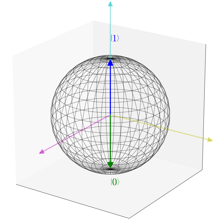
woooho

Qubit


Let's look at some quantum system described by a two-dimensional Hilbert space \ mathcal {H} ^ 2 and select in it some basis, the vectors of which are denoted as \ left | 0 \ right \ rangle and \ left | 1 \ right \ rangle . Inside the parentheses, the index of the basis vector in the binary number system is written, starting with zero without additional characters. Such designations will be very convenient. In this way,

\ left | 0 \ right \ rangle = \ begin {bmatrix} 1 \\ 0 \ end {bmatrix}, \; \ left | 1 \ right \ rangle = \ begin {bmatrix} 0 \\ 1 \ end {bmatrix},

and arbitrary vector \ left | \ psi \ right \ rangle \ in \ mathcal {H} ^ 2 can be expressed as follows:

\ left | \ psi \ right \ rangle = \ alpha \ left | 0 \ right \ rangle + \ beta \ left | 1 \ right \ rangle,

Where \ alpha and \ beta - some complex numbers such that \ vert \ alpha \ vert ^ 2 + \ vert \ beta \ vert ^ 2 = 1 (remember the interpretation of the decomposition coefficients and the normalization condition from the previous section). So, such a simple quantum system is called a qubit ( quantum bit , qbit ). A qubit is an analogue of a classic bit in a quantum computation model. It is easy to see that the space of all possible states of a single qubit \ mathcal {H} ^ 2 is a three-dimensional sphere, called the Bloch sphere, where \ left | 0 \ right \ rangle corresponds to the lower pole, and \ left | 1 \ right \ rangle - top.

sphere


Register


A single qubit, like a single bit, is too boring, so we immediately consider the superposition of several qubits. Such a superposition is called a quantum register ( quantum register , qregister ) of n qubits. For example, a quantum register of 2 qubits will be described by the space \ mathcal {H} ^ 4 and have 4 basic states:

\ left | 00 \ right \ rangle = \ left | 0 \ right \ rangle \ otimes \ left | 0 \ right \ rangle = \ begin {bmatrix} 1 \\ 0 \\ 0 \\ 0 \ end {bmatrix},

\ left | 01 \ right \ rangle = \ left | 0 \ right \ rangle \ otimes \ left | 1 \ right \ rangle = \ begin {bmatrix} 0 \\ 1 \\ 0 \\ 0 \ end {bmatrix},

\ left | 10 \ right \ rangle = \ left | 1 \ right \ rangle \ otimes \ left | 0 \ right \ rangle = \ begin {bmatrix} 0 \\ 0 \\ 1 \\ 0 \ end {bmatrix},

\ left | 11 \ right \ rangle = \ left | 1 \ right \ rangle \ otimes \ left | 1 \ right \ rangle = \ begin {bmatrix} 0 \\ 0 \\ 0 \\ 1 \ end {bmatrix}.

Accordingly, any state of such a register \ left | \ phi \ right \ rangle \ in \ mathcal {H} ^ 4 can be represented as

\ left | \ phi \ right \ rangle = \ alpha_1 \ left | 00 \ right \ rangle + \ alpha_2 \ left | 01 \ right \ rangle + \ alpha_3 \ left | 10 \ right \ rangle + \ alpha_4 \ left | 11 \ right \ rangle,

Where \ vert \ alpha_1 \ vert ^ 2 + \ vert \ alpha_2 \ vert ^ 2 + \ vert \ alpha_3 \ vert ^ 2 + \ vert \ alpha_4 \ vert ^ 2 = 1 . Notice that in our notation, a basis vector with a unit on k the second place is indicated by a number k recorded in binary form.

Further similar. Quantum register of m qubits will be described 2 ^ m -dimensional Hilbert space \ mathcal {H} ^ {2 ^ m} to have 2 ^ m basic states formed in a similar way. Without delay, let's learn how to emulate quantum registers:

 import numpy as np class QRegister: def __init__(self, n_qbits, init): self._n = n_qbits assert len(init) == self._n self._data = np.zeros((2 ** self._n), dtype=np.complex64) self._data[int('0b' + init, 2)] = 1 

3 lines of code to create a quantum register is not at all difficult, agree. You can use this way:

 a = QRegister(1, '0') # |0> b = QRegister(1, '1') # |1> c = QRegister(3, '010') # |010> 

The quantum algorithm includes:

  1. Initialization of the quantum register;
  2. A set of unitary transformations over it;
  3. Measurement result.

Measurement


We figured out the first item and learned how to emulate it, now let's learn how to emulate the last one: measurement. As you remember, the squares of the state vector coefficients physically mean the probabilities of transition to this state. In accordance with this, we are implementing a new method in the QRegister class:

 def measure(self): probs = np.real(self._data) ** 2 + np.imag(self._data) ** 2 states = np.arange(2 ** self._n) mstate = np.random.choice(states, size=1, p=probs)[0] return f'{mstate:>0{self._n}b}' 

We generate probabilities of probs choosing one of 2 ^ n states and randomly select it using np.random.choice . It remains only to return the binary string with the corresponding number of padding zeros. It is obvious that for basic states the answer will always be the same and equal to this state itself. Check:

 >>> QRegister(1, '0').measure() '0' >>> QRegister(2, '10').measure() '10' >>> QRegister(8, '01001101').measure() '01001101' 

Almost everything is ready to solve our problem! It remains only to learn how to influence the quantum registers. We already know that this can be done by unitary transformations.In quantum informatics, the unitary transformation is called a gate ( quantum gate , qgate , gate ).

Gates


In this article, we consider only a small number of the most basic gates, which will be useful to us. In fact, they are much more.

Unit


A single gate is the easiest one to look at. Its matrix is ​​as follows:

I = \begin{bmatrix}
    1 & 0\\
    0 & 1
\end{bmatrix}.

It does not change the qubit on which it acts:

I \left| 0 \right\rangle = \left| 0 \right\rangle,\; I \left| 1 \right\rangle = \left| 1 \right\rangle, \; I \left| \psi \right\rangle = \left| \psi \right\rangle,

However, you should not consider it useless - we will need it more than once.

Gate Hadamard


H = \frac{1}{\sqrt{2}}
\begin{bmatrix}
1 & 1\\
1 & -1
\end{bmatrix}

It is easy to verify that the matrix is ​​unitary:

H H^\dagger = \frac{1}{\sqrt{2}}
\begin{bmatrix}
1 & 1\\
1 & -1
\end{bmatrix} \cdot \frac{1}{\sqrt{2}}
\begin{bmatrix}
1 & 1\\
1 & -1
\end{bmatrix} = \frac{1}{2} \begin{bmatrix}
2 & 0\\
0 & 2
\end{bmatrix} = I.

Consider the effect of Hadamard gate on basic qubits:

H \left| 0 \right\rangle = \frac{1}{\sqrt{2}}
\begin{bmatrix}
1 & 1\\
1 & -1
\end{bmatrix}
\begin{bmatrix}
1\\
0
\end{bmatrix} = \frac{1}{\sqrt{2}}
\begin{bmatrix}
1\\
1
\end{bmatrix} = \frac{1}{\sqrt{2}} (\left| 0 \right\rangle + \left| 1 \right\rangle),

H \left| 1 \right\rangle = \frac{1}{\sqrt{2}}
\begin{bmatrix}
1 & 1\\
1 & -1
\end{bmatrix}
\begin{bmatrix}
0\\
1
\end{bmatrix} = \frac{1}{\sqrt{2}}
\begin{bmatrix}
1\\
-1
\end{bmatrix} = \frac{1}{\sqrt{2}} (\left| 0 \right\rangle - \left| 1 \right\rangle).

Or in general terms [1]:

H \left| x \right\rangle = \frac{1}{\sqrt{2}} \sum_{y \in \lbrace 0,1 \rbrace} (-1)^{x \cdot y} \left| y \right\rangle.

As you can see, Hadamard's gate translates any baseline state into equally probable - when measuring with equal probability, you can get any result.
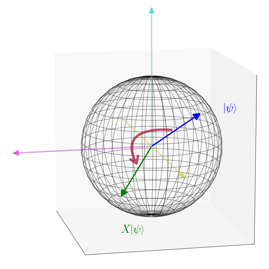
Gates of Pauli


Three extremely important gates to which the matrices introduced by Wolfgang Pauli correspond:

X =
\begin{bmatrix}
0 & 1\\
1 & 0
\end{bmatrix},\;
Y =
\begin{bmatrix}
0 & -i\\
i & 0
\end{bmatrix},\;
Z =
\begin{bmatrix}
1 & 0\\
0 & -1
\end{bmatrix}.

Gate is Xalso called NOT-gate:

X \left| 0 \right\rangle = \left| 1 \right\rangle, \; X \left| 1 \right\rangle = \left| 0 \right\rangle,

and its geometrical use is equivalent to a rotation on the Bloch sphere by \piradians around an axisx .

X gate

Gates Y and Zsimilar to the gate, Xwith the exception that the rotation is performed around the corresponding axis.

There is a theorem according to which with the help of gatesI , X , Y and Z Any one quit gate can be expressed. For example:

H = \frac{1}{\sqrt{2}}\big(X + Z\big),

where you can see that Hadamard gate geometrically means rotation on \piradians around the axis\frac{x + z}{\sqrt{2}} .

We implement all the considered gates in Python. To do this, create another class:

 class QGate: def __init__(self, matrix): self._data = np.array(matrix, dtype=np.complex64) assert len(self._data.shape) == 2 assert self._data.shape[0] == self._data.shape[1] self._n = np.log2(self._data.shape[0]) assert self._n.is_integer() self._n = int(self._n) 


And in the class QRegisterwe add the operation of applying the gate:

 def apply(self, gate): assert isinstance(gate, QGate) assert self._n == gate._n self._data = gate._data @ self._data 


And create already known to us gates:

 I = QGate([[1, 0], [0, 1]]) H = QGate(np.array([[1, 1], [1, -1]]) / np.sqrt(2)) X = QGate([[0, 1], [1, 0]]) Y = QGate([[0, -1j], [1j, 0]]) Z = QGate([[1, 0], [0, -1]]) 

Heads or tails?


coin

Let us consider, for example, the simplest quantum algorithm: it will generate a random bit - zero or one, eagle or tails. It will be the most honest coin in the universe - the result will be known only when measuring, and the nature of randomness is sewn into the very foundation of the universe and cannot be influenced by it in any way.

For the algorithm we need only one qubit. Let it be in the initial moment of time\left| 0 \right\rangle :

\left| 0 \right\rangle = \begin{bmatrix}
1\\
0
\end{bmatrix}.

Now apply the Hadamard gate to it Hto get the state

H \left| 0 \right\rangle = \frac{1}{\sqrt{2}}
\begin{bmatrix}
1\\
1
\end{bmatrix}.

If we now measure the resulting system, with probability \Big\vert \frac{1}{\sqrt{2}} \Big\vert^2 = \frac{1}{2}it will be able \left| 0 \right\rangleand with exactly the same probability as\left| 1 \right\rangle .It remains only to record the result.

Let's check the algorithm by emulating it on our classic computer:

 from quantum import QRegister, H def quantum_randbit(): a = QRegister(1, '0') a.apply(H) return a.measure() for i in range(32): print(quantum_randbit(), end='') print() 

Results:

 âžś python example-randbit.py 11110011101010111010011100000111 âžś python example-randbit.py 01110000111100011000101010100011 âžś python example-randbit.py 11111110011000001101010000100000 

All the above algorithm can be written with a pair of formulas:

\left| q_0 \right\rangle = \left| 0 \right\rangle\\
\left| q_1 \right\rangle = H \left| q_0 \right\rangle\\
r = measure(\left| q_1 \right\rangle)

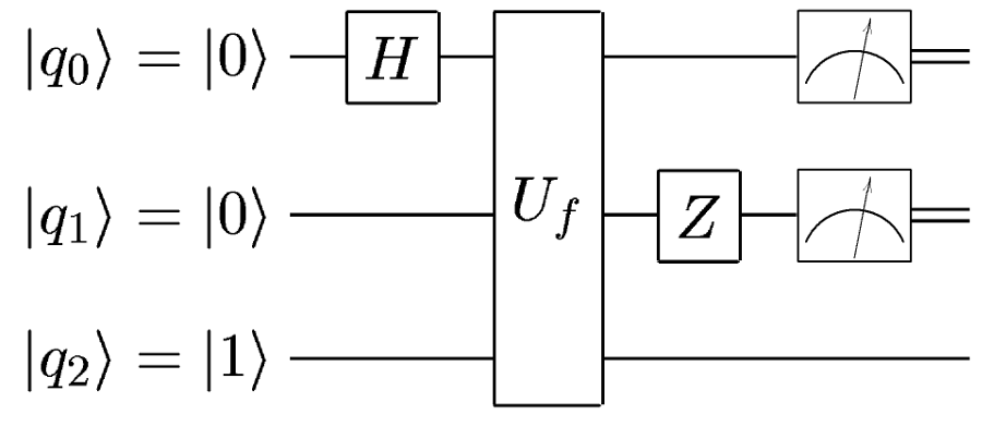
However, it is not very convenient to work with such a record: the structure of the list is a sequence of actions that is well suited for classical algorithms, is not applicable in the quantum case: here we have neither cycles nor conditions, only state flow forward (and sometimes back) in time . Therefore, quantum schemes are widely used to describe algorithms in quantum computer science. Here is a diagram of the above algorithm:
simple

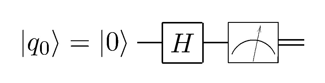
On the left is always indicated the initial state of the system. Unitary transformations performed on this state are indicated in the rectangles, and at the end a measuring instrument icon is placed on all or on several qubits - a measurement operation. There is also a “syntactic sugar” for some multi-qubit transformations in the form of points, ramifications, and circles. And that's all. If you can distinguish a square from a triangle and a circle, you will easily understand any scheme of the quantum algorithm.

holes

More qubits to qubit god


And what if we work not with one qubit, but with their whole register? And, let's say, we want to apply the gate only to one qubit? The properties of the tensor product come to the rescue. By definition, the tensor product of an operatorA: V \to W and B: X \to Y :

(A \otimes B)(v \otimes x) = Av \otimes Bx,

Where v \in V , x \in X . Then:

(A \otimes I)(v \otimes x) = Av \otimes Ix = Av \otimes x,

that is, it doesn't matter if you apply the gate to one qubit, and then connect it with the second one and get a quantum register, or apply the operator to the whole register A \otimes I .Similarly, if we want to apply the operator Aonly to the second qubit, we can apply the operator to the whole registerI \otimes A . This means that this scheme:

example0

Completely similar to this:

example1

Only single gates are omitted for convenience.

And if we, on the contrary, want to apply the gate to several qubits at once? Again, from the definition of a tensor product, for this we can apply this gate to them, the tensor multiplied by itself the necessary number of times:

Hv \otimes Hx = (H \otimes H) (v \otimes x) = H^{\otimes2} (v \otimes x).

A^{\otimes n} means tensor exponentiation. By the way \left| \psi \right \rangle^{\otimes n} for brevity, recorded as \left| \psi^n \right \rangle . In this way,

H^{\otimes n} \left| 0^n \right \rangle

means: napply a Hadamard transform to each qubit of the quantum register of zero qubits.

Add a tensor product and exponentiation to ours QGate:

 def __matmul__(self, other): return QGate(np.kron(self._data, other._data)) def __pow__(self, n, modulo=None): x = self._data.copy() for _ in range(n - 1): x = np.kron(x, self._data) return QGate(x) 

Quantum oracle


Each binary function f : \{0, 1\}^n \to \{0, 1\}corresponds to a single multi-qubit gate of dimension n + 1, which is denoted U_fand called the quantum oracle for this function. It contains all the information about the function fand “allows” to simultaneously call it on all of its possible arguments.

Why is its dimensionn + 1 ?The thing is that according to another fundamental property of quantum computing, information is not lost in them and they are reversible in time. If we call a function in the classical computational model f(x, y) = x \oplus yand get the result, then we can’t tell with one of which arguments the function was called and, accordingly, we cannot invert the computations in time.

diagram0


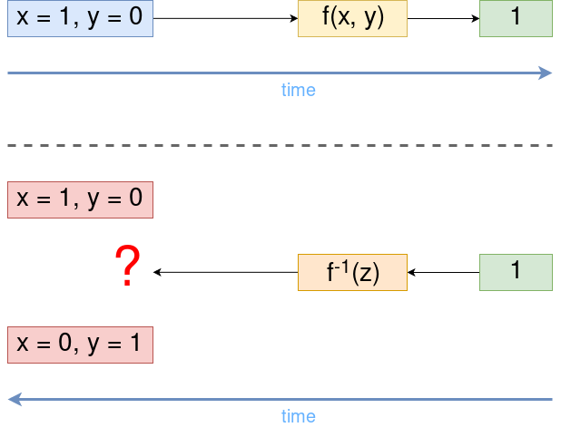
One way to avoid this is to memorize the arguments with which the function was invoked.

diagram1


The same thing happens in the quantum model of computation, only there it is embedded in their very nature - without saving the complete information, it is impossible to build a unitary transformation.

A quantum oracle is U_fdefined as a unitary transformation that transforms a state \left| x \right \rangle \left| y \right \rangleinto a state\left| x \right \rangle \left| y \oplus f(x) \right \rangle where nqubits, denoted x, carry information about the function argument and remain unchanged, and the only qubit y- its result. \oplusdenotes addition modulo 2.

Let's look at an example. Suppose we want to build an oracle for a function of one argumentf(x) = x .Hence, the corresponding operator U_fwill be two-qubit and can be described by a square matrix of dimension2^2 = 4 . In accordance with the rule described above, let's see into which states all the basic register states should go:

\left| 00 \right \rangle  = \left| 0 \right \rangle \left| 0 \right \rangle \to \left| 0 \right \rangle \left| 0 \oplus f(0) \right \rangle = \left| 00 \right \rangle

\left| 01 \right \rangle  = \left| 0 \right \rangle \left| 1 \right \rangle \to \left| 0 \right \rangle \left| 0 \oplus f(1) \right \rangle = \left| 01 \right \rangle

\left| 10 \right \rangle  = \left| 1 \right \rangle \left| 0 \right \rangle \to \left| 1 \right \rangle \left| 1 \oplus f(0) \right \rangle = \left| 11 \right \rangle

\left| 11 \right \rangle  = \left| 1 \right \rangle \left| 1 \right \rangle \to \left| 1 \right \rangle \left| 1 \oplus f(1) \right \rangle = \left| 10 \right \rangle

, i - i - . i - j - , , j - , i - . {00}_2 = 0 and {01}_2 = 1 {10}_2 = 3 and {11}_2 = 4 . Then U_f :

U_f = \begin{bmatrix}
1 & 0 & 0 & 0\\
0 & 1 & 0 & 0\\
0 & 0 & 0 & 1\\
0 & 0 & 1 & 0\\
\end{bmatrix}.

:

\begin{bmatrix}
1 & 0 & 0 & 0\\
0 & 1 & 0 & 0\\
0 & 0 & 0 & 1\\
0 & 0 & 1 & 0\\
\end{bmatrix}\begin{bmatrix}
x_{00} \\
x_{01} \\
x_{10} \\
x_{11} \\
\end{bmatrix} = \begin{bmatrix}
x_{00} \\
x_{01} \\
x_{11} \\
x_{10} \\
\end{bmatrix}.

. :

 def U(f, n): m = n + 1 U = np.zeros((2**m, 2**m), dtype=np.complex64) def bin2int(xs): r = 0 for i, x in enumerate(reversed(xs)): r += x * 2 ** i return r for xs in product({0, 1}, repeat=m): x = xs[:~0] y = xs[~0] z = y ^ f(*x) instate = bin2int(xs) outstate = bin2int(list(x) + [z]) U[instate, outstate] = 1 return QGate(U) 

Still remains


, , . , , , — . 1985 , 1992 . :
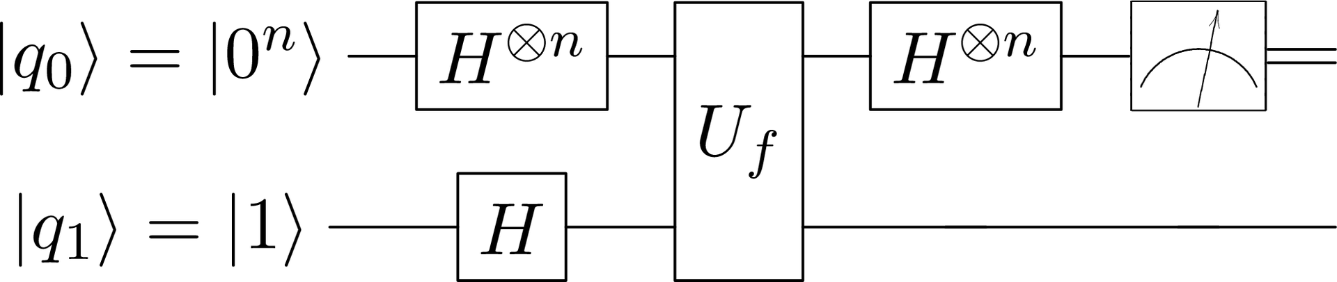
dj

0, , — . :

 from quantum import QRegister, H, I, U def is_constant(f, n): q = QRegister(n + 1, '0' * n + '1') q.apply(H ** (n + 1)) q.apply(U(f, n)) q.apply(H ** n @ I) if q.measure()[:~0] == '0' * n: return True else: return False 

:

 def f1(x): return x def f2(x): return 1 def f3(x, y): return x ^ y def f4(x, y, z): return 0 print('f(x) = x is {}'.format('constant' if is_constant(f1, 1) else 'balansed')) print('f(x) = 1 is {}'.format('constant' if is_constant(f2, 1) else 'balansed')) print('f(x, y) = x ^ y is {}'.format('constant' if is_constant(f3, 2) else 'balansed')) print('f(x, y, z) = 0 is {}'.format('constant' if is_constant(f4, 3) else 'balansed')) 

Result:

 f(x) = x is balansed f(x) = 1 is constant f(x, y) = x ^ y is balansed f(x, y, z) = 0 is constant 

Works. Wonderful. ? .

H [1]:

H^{\otimes n} \left|x_1, x_2, \ldots, x_n\right\rangle =

(by the property of a tensor product)

= H \left| x_1 \right\rangle \otimes H \left| x_2 \right\rangle \otimes \dots \otimes H \left| x_n \right\rangle =

(applicable to every single qubit)

=\frac{1}{\sqrt{2^n}} \Big(\sum \limits_{y_1 \in \lbrace 0,1 \rbrace} (-1)^{x_1 \cdot y_1} \left| y_1 \right\rangle \otimes \sum \limits_{y_2 \in \lbrace 0,1 \rbrace} (-1)^{x_2 \cdot y_2} \left| y_2 \right\rangle \otimes \ldots \otimes \sum \limits_{y_n \in \lbrace 0,1 \rbrace} (-1)^{x_n \cdot y_n} \left| y_n \right\rangle \Big) =

(we take out -1 for the sign of the tensor product)

=\frac{1}{\sqrt{2^n}} \sum \limits_{(y_1, y_2, \ldots, y_n) \in \lbrace 0,1 \rbrace^n} (-1)^{x_1 \cdot y_1 \oplus x_2 \cdot y_2 \oplus \dots \oplus x_n \cdot y_n} \left| {y_1 y_2 \ldots y_n} \right\rangle =

(redefine for compactness)

=\frac{1}{\sqrt{2^n}} \sum \limits_{y \in \lbrace 0,1 \rbrace^n} (-1)^{(x, y)} \left| y \right\rangle,

Where \oplus- addition modulo 2, and (x, y)- scalar product modulo 2.

At the initial moment of time the system is in a state \left| {q_0} \right\rangle \left| {q_1} \right\rangle = \left| 0 \right\rangle^{\otimes n} \left| 1 \right\rangleand under the action of the Hadamard transform will go into

H^{\otimes n} \left| 0 \right\rangle^{\otimes n} (H \left| 1 \right\rangle) = \frac{1}{\sqrt{2^{n+1}}}\displaystyle\sum_{x=0}^{2^n} \left| x \right\rangle \big(\left| 0 \right\rangle - \left|1 \right\rangle \big).

Oracle will U_fput the system in state

\frac{1}{\sqrt{2^{n+1}}}\displaystyle\sum_{x=0}^{2^n} \left| x \right\rangle \Big(\left| {f(x)} \right\rangle \oplus \big(\left| 0 \right\rangle - \ \left| 1 \right\rangle \big) \Big) = \frac{1}{\sqrt{2^{n+1}}}\displaystyle\sum_{x=0}^{2^n} \left| x \right\rangle \Big( \left| {f(x)} \right\rangle - \left| {f(x) \oplus 1} \right\rangle \Big).

Note that if at some fixed argument the xfunction f (x)takes the value 0, then the coefficient before \left| x \right\ranglewill not change, otherwise it will change the sign. Based on this observation, you can rewrite the current state as

\frac{1}{\sqrt{2^{n+1}}}\displaystyle\sum_{x=0}^{2^n} (-1)^{f(x)} \left| x \right\rangle \big( \left| 0 \right\rangle - \left| 1 \right\rangle \big).

n ,

H^{\otimes n} \Big( \frac{1}{\sqrt{2^n}}\displaystyle\sum_{x=0}^{2^n} (-1)^{f(x)} \left| x \right\rangle \Big) = \frac{1}{2^n}\displaystyle\sum_{y=0}^{2^n} \Big( \displaystyle\sum_{x=0}^{2^n} (-1)^{f(x) + x \cdot y} \Big) \left| y \right\rangle.

x \cdot 0^n = 0 , \left| {0^n} \right\rangle equals

\frac{1}{2^n}\displaystyle\sum_{x=0}^{2^n} (-1)^{f(x)} = 
\begin{cases}
   1 &\text{,  $f(x)$ }\\
   0 &\text{,  $f(x)$ }
\end{cases}.

That's all. , - «» — -. , , :

.

→ GitHub

Thanks for reading! , , , . .

Literature


PS : — . Roman Parpalak upmath.me , .

Source: https://habr.com/ru/post/321292/


All Articles