Interesting clustering algorithms, part one: Affinity propagation
Part One - Affinity Propagation
Part Two - DBSCAN
Part Three - Time Series Clustering
Part Four - Self-Organizing Maps (SOM)
Part Five - Growing Neural Gas (GNG)
If you ask the novice data analyst what classification methods he knows, you will probably list a fairly decent list: statistics, trees, SVM, neural networks ... But if you ask about clustering methods, you will most likely get “k-means the same!” It is this golden hammer that is considered in all machine learning courses. Often, it does not even reach its modifications (k-medians) or connected-graph methods.
It's not that k-means is so bad, but its result is almost always cheap and angry. There are more advanced ways of clustering, but not everyone knows which one to use, and very few understand how they work. I would like to lift the veil of secrecy over some algorithms. Let's start with Affinity propagation.
')
It is assumed that you are familiar with the classification of clustering methods , and also have used k-means and know its pros and cons. I will try not to go very deeply into theory, but to try to convey the idea of the algorithm in simple language.
Affinity propagation (AP, also known as proximity propagation method) receives as input a similarity matrix between dataset elements t e x t b f S = N t i m e s N and returns the set of labels assigned to these elements. Without further ado, I immediately put the algorithm on the table:
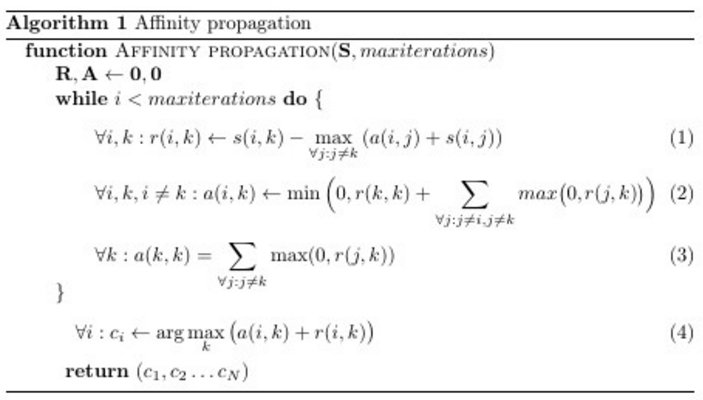
Ha, it would be something to lay out. Only three lines, if we consider the main loop; (4) is obviously the label assignment rule. But not everything is so simple. Most programmers are not at all clear what these three lines are doing with matrices. t e x t b f S , t e x t b f R and t e x t b f A . An official article explains that t e x t b f R and t e x t b f A - matrixes of “responsibility” and “accessibility”, respectively, and that in the cycle there is a “message exchange” between potential cluster leaders and other points. Honestly, this is a very superficial explanation, and it is not clear either the purpose of these matrices or how and why their values change. Trying to figure out is likely to lead you somewhere here . Good article, but it is difficult for an unprepared person to endure a whole monitor screen full of formulas.
So I will start from the other end.
In a certain space, in a certain state, dots live. Dots have a rich inner world, but there is some rule s ( i , k ) , by which they can tell how much a neighbor is like them. Moreover, they already have a table. t e x t b f S where everything is recorded s ( i , k ) and it almost never changes.
It’s boring for one to live in the world, so the points want to gather in hobby groups. Circles are formed around the leader (exemplar), who represents the interests of all members of the partnership. Each point would like to see the leader of someone who most closely resembles her, but is willing to put up with other candidates if they like many others. It should be added that the points are quite modest: everyone thinks that someone else should be the leader. You can reformulate their low self-esteem as follows: each point believes that when it comes to grouping, it does not resemble itself ( s ( k , k ) < 0 ). Convince the point to become a leader, can either collective encouragement from similar comrades, or, conversely, if the society does not have absolutely no one like her.
The points do not know in advance what the teams will be or their total number. The union goes from the top down: first, the dots cling to the presidents of the groups, then they only ponder who else supports the same candidate. The choice of a point as a leader is influenced by three parameters: similarity (it has already been said about it), responsibility and accessibility. Responsibility (responsibility, table t e x t b f R with elements r ( i , k ) ) is responsible for how i wants to see k their leader. Responsibility is assigned by each point to the candidate for the group leaders. Availability (availability, table t e x t b f A , with elements a ( i , k ) ) - there is a response from a potential leader k , how good k ready to represent interests i . Responsibility and accessibility of a point is calculated including for oneself. Only when self-responsibility is great (yes, I want to represent my interests) and self-accessibility (yes, can I represent my interests), i.e. a(k,k)+r(k,k)>0 , the point can overcome innate self-doubt. Ordinary points eventually join the leader, for whom they have the greatest amount a(i,k)+r(i,k) . Usually at the very beginning, textbfR= textbf0 and textbfA= textbf0 .
Let's take a simple example: points X, Y, Z, U, V, W, whose whole inner world is love for cats, K . X is allergic to cats, we assume for him K=−2 , Y refers to them cool, K=−1 , and Z is just not up to them, K=0 . U has four cats at home ( K=4 ), V - five ( K=5 ), and W has forty ( K=40 ). We define the difference as the absolute value of the difference K . X is unlike Y by one conditional point, and U is as much as six. Then the similarity s(i,k) - this is just a minus difference. It turns out that the points with zero similarity are exactly the same; more negative s(i,k) the more points are different . A little counterintuitive, but oh well. The size of “self-similarity” in the example is estimated at 2 points ( s(k,k)=−2 ).
So, in the first step, every point i puts the responsibility on everyone k (including on itself) in proportion to the similarity between i and k and inversely proportional to the similarity between i and the most similar vector except k ((1) c a(i,j)=0 ). In this way:
If a r(i,k)>0 then i would like to k was her representative. r(k,k)>0 means itself k wants to be the founder of the team, r(k,k)<0 - what k wants to belong to another team.
Returning to the example: X places responsibility on Y −1−(−2)=1 score, on Z - −2−(−1)=−1 score, U - −6−(−1)=−$ and myself −2−(−1)=−1 . X, in general, is not opposed to Z being the leader of the cat-hater group, if Y does not want to be him, but he is unlikely to communicate with U and V, even if they form a large team. W is so unlike all the other points that she can do nothing but put responsibility on the size. −2−(−35)=$3 points only on yourself.
Then the points begin to think how ready they are to be a leader (available, available, for leadership). Accessibility for oneself (3) is made up of all the positive responsibility, the “votes” given to the point. For k no matter how many points they think it will be bad to represent them. For her, the main thing is that at least someone thinks that she will represent them well. Availability k for i depends on how much k ready to present himself and on the number of positive reviews about him (2) (someone else also believes that he will be an excellent representative of the team). This value is limited to zero from above in order to reduce the influence of points about which too many people think well, so that they do not combine even more points into one group and the cycle does not go out of control. The smaller r(k,k) the more votes you need to collect k so that a(i,k) was equal to 0 (i.e., this point was not against taking under its wing also i ).
A new election phase begins, but now textbfA neq textbf0 . Recall that a(k,k) geq0 , but a(i,k) leq0,i neqk . This has a different effect on r(i,k)
Accessibility leaves points in the competition that are either ready to stand up for themselves (W, a(i,i)=0 , but it does not affect (1), since even taking into account the amendment, W is very far from the other points) or those for which others are ready to stand (Y, in (3) it has a term from X and Z). X and Z, which are not strictly best resemble someone, but still resemble someone, are eliminated from the competition. This affects the distribution of responsibility, which affects the distribution of availability, and so on. In the end, the algorithm stops - a(i,k) stop changing. X, Y and Z unite in a company around Y; are friends of U and V with U as a leader; W well and with 40 cats.
We rewrite the decision rule to get another look at the decision rule of the algorithm. We use (1) and (3). Denote tildes(i,k)=a(i,k)+s(i,k) - similarity with the correction that k talks about his commanding abilities i ; tilded(i,k)=− tildes(i,k) - dissimilarity i - k with the amendment.
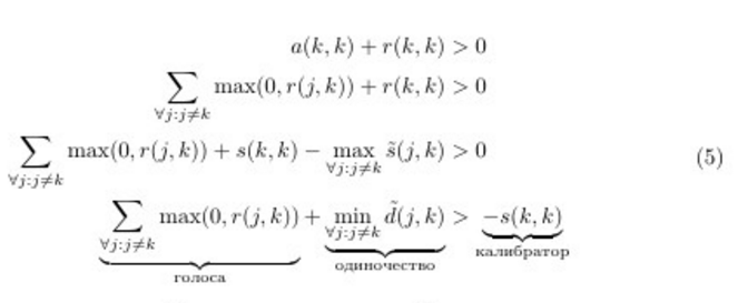
Approximately what I formulated at the beginning. It is clear from this that the less confident the points are, the more “votes” must be collected or the more unlike the others you need to be in order to become a leader. Those. the smaller s(k,k) the bigger the groups are.
Well, I hope you have gained some intuitive insight into how the method works. Now a little more serious. Let's talk about the nuances of the algorithm.
Clustering can be represented as a discrete maximization problem with constraints. Let a function of similarity be given on the set of elements s(i,j) . Our task is to find such a vector of labels. \ mathbf {c} = \ {c_1, c_2 ... c_N \}, c_i \ in \ {1 \ dots N \} which maximizes the function
Where delta(ck) - member limiter equal to − infty if point exists i that chose a point k its leader ( ci=k ), but myself k the leader does not consider himself ( ck neqk ). The bad news: finding the perfect mathbfc - This is an NP-complex task, known as the object allocation problem. Nevertheless, there are several approximate algorithms for its solution. In methods that interest us si , ci and deltai are represented by the vertices of a bipartite graph, after which information is exchanged between them, which makes it possible from the probabilistic point of view to evaluate which label is better suited for each element. See the output here . About the distribution of messages in bipartite graphs, see here . In general, proximity propagation is a special case (rather, narrowing) of cyclic belief propagation (loopy belief propagation, LBP, see here ), but instead of a sum of probabilities (Sum-Product subtype) in some places we take only the maximum (Max-Product subtype) of them. Firstly, LBP-Sum-Product is an order of magnitude more difficult, secondly, it’s easier to deal with computational problems, thirdly, theorists say that it makes more sense for the clustering problem.
AP authors talk a lot about “messages” from one element of the graph to another. Such an analogy comes from the derivation of formulas through the dissemination of information in a graph. In my opinion, it is a bit confusing, because in the implementations of the algorithm there are no “point-to-point” messages, but there are three matrices textbfS , textbfR and textbfA . I would suggest the following interpretation:
Affinity propagation is deterministic. He has difficulty O(N2T) where N - the size of the data set, and T - the number of iterations, and takes O(N2) of memory. There are modifications of the algorithm for sparse data, but still the AP is very sad with the increase in the size of the dataset. This is a pretty serious drawback. But the distribution of proximity does not depend on the dimension of the data elements. So far there is no parallelized version of AP. The trivial parallelization in the form of a set of algorithm starts is not suitable due to determinism. In the official FAQ , it is written that there are no options with adding real-time data either, but I found just such an article.
There is an accelerated version of AP . The method proposed in the article is based on the idea that it is not necessary to calculate in general all updates of the accessibility and liability matrices, because all points in the thick of other points belong to instances far from them approximately equally.
If you want to experiment (keep it up!), I would suggest conjuring over formulas (1-5). Parts max(0,x) they look suspiciously similar to neural network ReLu. I wonder what happens if you use ELu. In addition, since you now understand the essence of what is happening in the cycle, you can add additional terms to the formulas that are responsible for the behavior you need. Thus, it is possible to “push” the algorithm towards clusters of a certain size or shape. You can also impose additional restrictions if it is known that some elements are more likely to belong to the same set. However, this is speculation.
Affinity propagation, like many other algorithms, can be interrupted ahead of time , if textbfR and textbfA stop updating. For this, almost all implementations use two values: the maximum number of iterations and the period with which the amount of updates is checked.
Affinity propagation is subject to computational oscillations in cases where there are several good clustering. To avoid problems, firstly, at the very beginning , a bit of noise is added to the similarity matrix (very, very little, so as not to affect determinism, in the sklearn-implementation of the order 10−16 ), and secondly, when updating textbfR and textbfA it is not a simple assignment that is used, but an assignment with an exponential smoothing . Moreover, the second optimization has a good effect on the quality of the result, but because of it the number of necessary iterations increases. T . Authors advise using a smoothing parameter. 0.5 l e q g a m m a < 1.0 with default value in 0.5 . If the algorithm does not converge or partially converges, you should increase g a m m a before 0.9 or until 0.95 with a corresponding increase in the number of iterations.
This is how a failure looks like - a bunch of small clusters surrounded by a ring of medium-sized clusters:
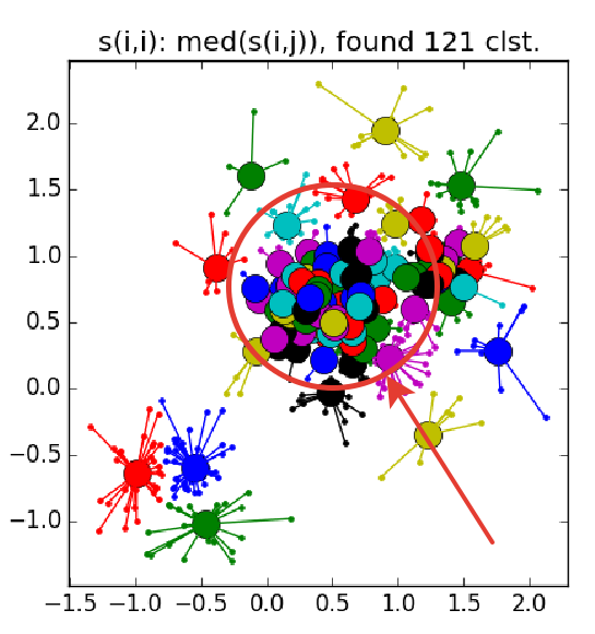
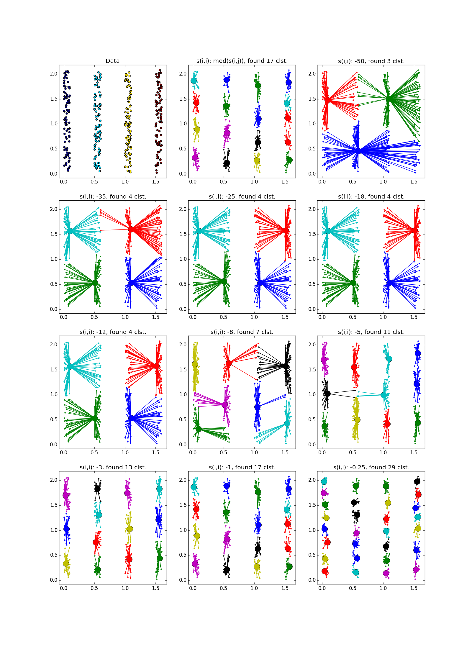
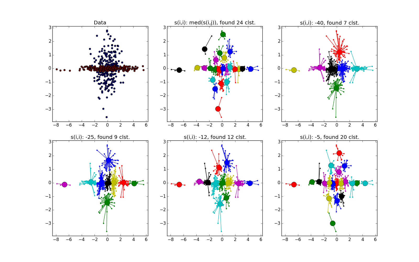
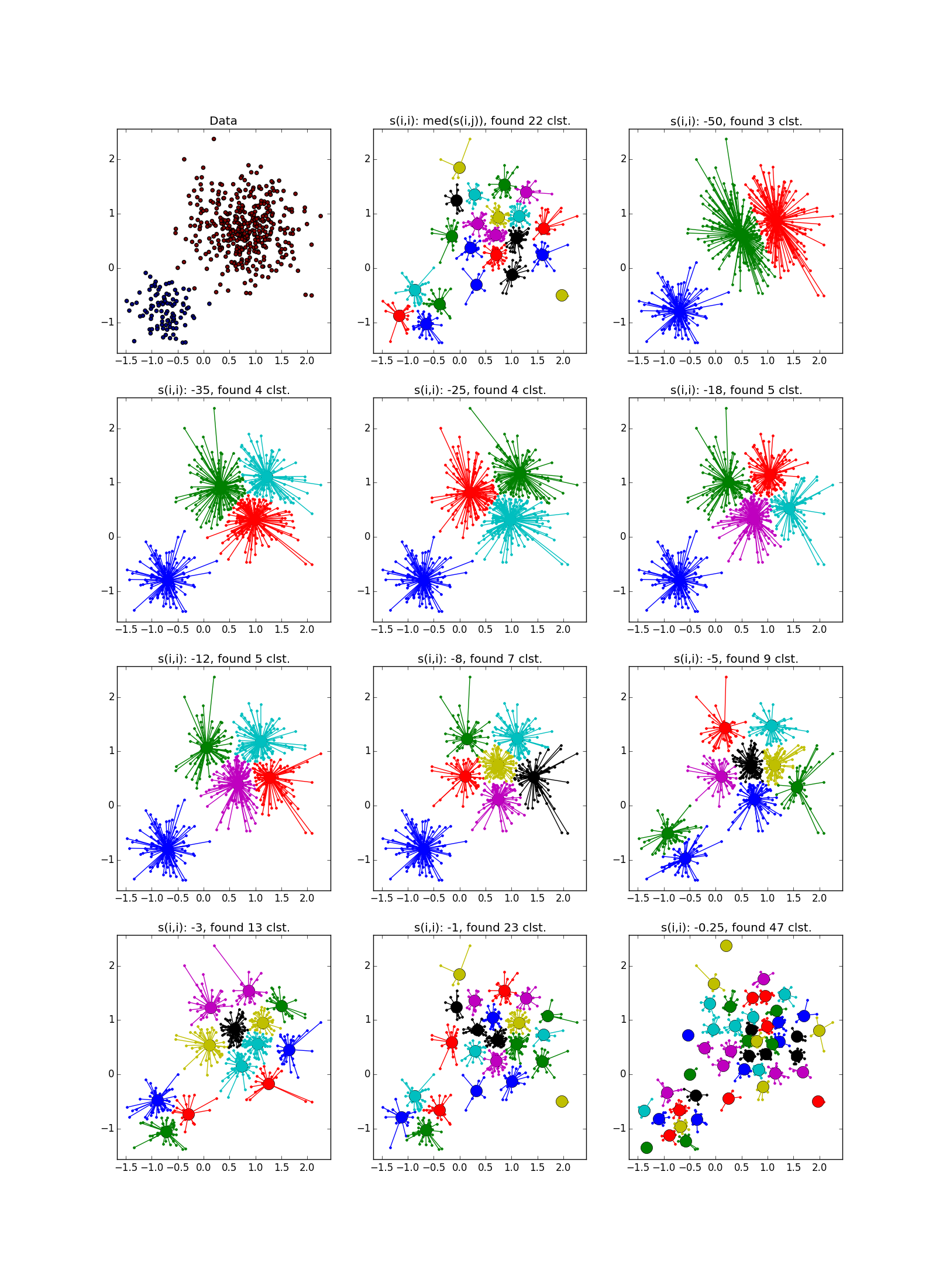
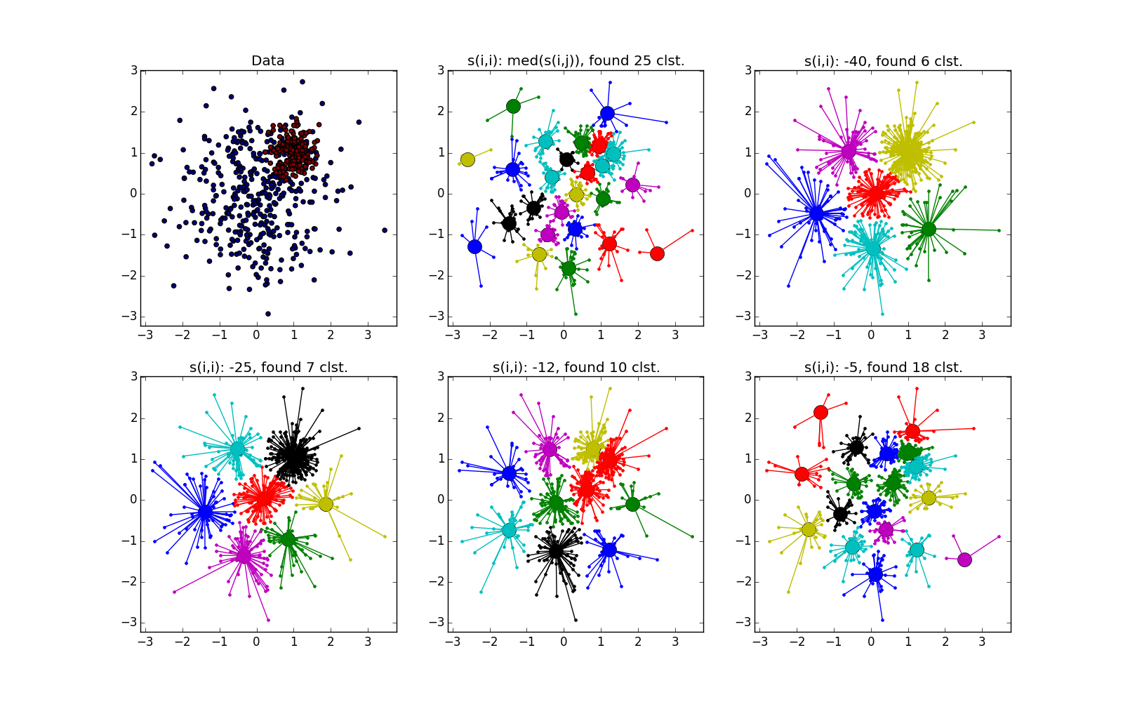
As already mentioned, instead of a predetermined number of clusters, the “self-similarity” parameter is used. s ( k , k ) ; the smaller s ( k , k ) the larger the clusters. There are heuristics for automatic adjustment of the value of this parameter: use the median for all s ( i , k ) for the greater number of clusters; 25 percentile or even at least s ( i , k ) - for less (you still have to customize, ha ha). If the self-similarity value is too small or too large, the algorithm will not produce any useful results at all.
As s ( i , k ) itself suggests to use the negative Euclidean distance between i and j , but no one limits you in choosing. Even in the case of dataset from the vectors of real numbers, you can try a lot of interesting things. In general, the authors argue that the function of similarity is not imposed any special restrictions ; it is not even necessary that the symmetry rule or the triangle rule be fulfilled. But it's worth noting that the more cunning you have s ( i , j ) , the less likely that the algorithm will converge to something interesting.
The sizes of clusters obtained during the proximity propagation vary within rather small limits, and if there are clusters of very different sizes in dataset, the AP can either skip small ones or count large ones for a few. Usually the second situation is less unpleasant - it is fixable. Therefore, the AP often needs to be post-processed - additional clustering of group leaders . Any other method is suitable, additional information about the task can help. It should be remembered that honest lonely standing points stand out their clusters; such emissions need to be filtered before post-processing.
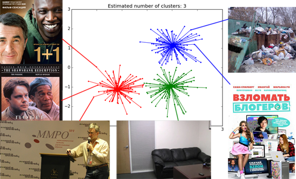
Fuh, the wall of the text is over, the wall of pictures has begun. Let's check Affinity propagation on different types of clusters.
Use Affinity propagation when
It is argued that various scientists have successfully used Affinity propagation for
In all these cases, the result was obtained better than with the help of k-means. Not that this is some kind of awesome result in itself. I don’t know if in all these cases there was a comparison with other algorithms. I plan to do this in future articles. Apparently, in real-life datasets, the ability to distribute proximity helps most of all with clusters of different geometric shapes.
Well, everything seems to be all. Next time we will consider some other algorithm and compare it with the method of proximity propagation. Good luck, Habr!
Part Two - DBSCAN
Part Three - Time Series Clustering
Part Four - Self-Organizing Maps (SOM)
Part Five - Growing Neural Gas (GNG)
If you ask the novice data analyst what classification methods he knows, you will probably list a fairly decent list: statistics, trees, SVM, neural networks ... But if you ask about clustering methods, you will most likely get “k-means the same!” It is this golden hammer that is considered in all machine learning courses. Often, it does not even reach its modifications (k-medians) or connected-graph methods.
It's not that k-means is so bad, but its result is almost always cheap and angry. There are more advanced ways of clustering, but not everyone knows which one to use, and very few understand how they work. I would like to lift the veil of secrecy over some algorithms. Let's start with Affinity propagation.
')
It is assumed that you are familiar with the classification of clustering methods , and also have used k-means and know its pros and cons. I will try not to go very deeply into theory, but to try to convey the idea of the algorithm in simple language.
Affinity propagation
Affinity propagation (AP, also known as proximity propagation method) receives as input a similarity matrix between dataset elements t e x t b f S = N t i m e s N and returns the set of labels assigned to these elements. Without further ado, I immediately put the algorithm on the table:
Ha, it would be something to lay out. Only three lines, if we consider the main loop; (4) is obviously the label assignment rule. But not everything is so simple. Most programmers are not at all clear what these three lines are doing with matrices. t e x t b f S , t e x t b f R and t e x t b f A . An official article explains that t e x t b f R and t e x t b f A - matrixes of “responsibility” and “accessibility”, respectively, and that in the cycle there is a “message exchange” between potential cluster leaders and other points. Honestly, this is a very superficial explanation, and it is not clear either the purpose of these matrices or how and why their values change. Trying to figure out is likely to lead you somewhere here . Good article, but it is difficult for an unprepared person to endure a whole monitor screen full of formulas.
So I will start from the other end.
Intuitive explanation
In a certain space, in a certain state, dots live. Dots have a rich inner world, but there is some rule s ( i , k ) , by which they can tell how much a neighbor is like them. Moreover, they already have a table. t e x t b f S where everything is recorded s ( i , k ) and it almost never changes.
It’s boring for one to live in the world, so the points want to gather in hobby groups. Circles are formed around the leader (exemplar), who represents the interests of all members of the partnership. Each point would like to see the leader of someone who most closely resembles her, but is willing to put up with other candidates if they like many others. It should be added that the points are quite modest: everyone thinks that someone else should be the leader. You can reformulate their low self-esteem as follows: each point believes that when it comes to grouping, it does not resemble itself ( s ( k , k ) < 0 ). Convince the point to become a leader, can either collective encouragement from similar comrades, or, conversely, if the society does not have absolutely no one like her.
The points do not know in advance what the teams will be or their total number. The union goes from the top down: first, the dots cling to the presidents of the groups, then they only ponder who else supports the same candidate. The choice of a point as a leader is influenced by three parameters: similarity (it has already been said about it), responsibility and accessibility. Responsibility (responsibility, table t e x t b f R with elements r ( i , k ) ) is responsible for how i wants to see k their leader. Responsibility is assigned by each point to the candidate for the group leaders. Availability (availability, table t e x t b f A , with elements a ( i , k ) ) - there is a response from a potential leader k , how good k ready to represent interests i . Responsibility and accessibility of a point is calculated including for oneself. Only when self-responsibility is great (yes, I want to represent my interests) and self-accessibility (yes, can I represent my interests), i.e. a(k,k)+r(k,k)>0 , the point can overcome innate self-doubt. Ordinary points eventually join the leader, for whom they have the greatest amount a(i,k)+r(i,k) . Usually at the very beginning, textbfR= textbf0 and textbfA= textbf0 .
Let's take a simple example: points X, Y, Z, U, V, W, whose whole inner world is love for cats, K . X is allergic to cats, we assume for him K=−2 , Y refers to them cool, K=−1 , and Z is just not up to them, K=0 . U has four cats at home ( K=4 ), V - five ( K=5 ), and W has forty ( K=40 ). We define the difference as the absolute value of the difference K . X is unlike Y by one conditional point, and U is as much as six. Then the similarity s(i,k) - this is just a minus difference. It turns out that the points with zero similarity are exactly the same; more negative s(i,k) the more points are different . A little counterintuitive, but oh well. The size of “self-similarity” in the example is estimated at 2 points ( s(k,k)=−2 ).
So, in the first step, every point i puts the responsibility on everyone k (including on itself) in proportion to the similarity between i and k and inversely proportional to the similarity between i and the most similar vector except k ((1) c a(i,j)=0 ). In this way:
- The nearest (most similar) point specifies the distribution of responsibility for all other points. The location of points beyond the first two so far affects only r(i,k) allotted to them and only to them.
- The responsibility placed on the nearest point also depends on the location of the second nearest.
- If within reach i there are several more or less similar candidates; those will be assigned the same responsibility.
- s(k,k) acts as a kind of limiter - if a point is too different from all the others, there is nothing left for it but to rely only on itself
If a r(i,k)>0 then i would like to k was her representative. r(k,k)>0 means itself k wants to be the founder of the team, r(k,k)<0 - what k wants to belong to another team.
Returning to the example: X places responsibility on Y −1−(−2)=1 score, on Z - −2−(−1)=−1 score, U - −6−(−1)=−$ and myself −2−(−1)=−1 . X, in general, is not opposed to Z being the leader of the cat-hater group, if Y does not want to be him, but he is unlikely to communicate with U and V, even if they form a large team. W is so unlike all the other points that she can do nothing but put responsibility on the size. −2−(−35)=$3 points only on yourself.
Then the points begin to think how ready they are to be a leader (available, available, for leadership). Accessibility for oneself (3) is made up of all the positive responsibility, the “votes” given to the point. For k no matter how many points they think it will be bad to represent them. For her, the main thing is that at least someone thinks that she will represent them well. Availability k for i depends on how much k ready to present himself and on the number of positive reviews about him (2) (someone else also believes that he will be an excellent representative of the team). This value is limited to zero from above in order to reduce the influence of points about which too many people think well, so that they do not combine even more points into one group and the cycle does not go out of control. The smaller r(k,k) the more votes you need to collect k so that a(i,k) was equal to 0 (i.e., this point was not against taking under its wing also i ).
A new election phase begins, but now textbfA neq textbf0 . Recall that a(k,k) geq0 , but a(i,k) leq0,i neqk . This has a different effect on r(i,k)
- i=k . Then a(k,k) geq0 does not matter, and in (1) everything −max( dots) the right side will be no less than they were in the first step. a(i,j)<0 as a matter of fact, alienates the point i from j . The self-responsibility of the point rises from the fact that the best candidate from her point of view has bad reviews.
- i neqk . Both effects come out here. This case splits into two:
- a(i,j)+s(i,j),i neqj - max. Same as in case 1, but the responsibility imposed on the point increases k
- a(i,i)+s(i,i) - max. Then −max( dots) will be no more than the first step r(i,k) decreases. If we continue the analogy, then it is as if the point, which already thought about whether to become its leader, would have received additional approval.
- a(i,j)+s(i,j),i neqj - max. Same as in case 1, but the responsibility imposed on the point increases k
Accessibility leaves points in the competition that are either ready to stand up for themselves (W, a(i,i)=0 , but it does not affect (1), since even taking into account the amendment, W is very far from the other points) or those for which others are ready to stand (Y, in (3) it has a term from X and Z). X and Z, which are not strictly best resemble someone, but still resemble someone, are eliminated from the competition. This affects the distribution of responsibility, which affects the distribution of availability, and so on. In the end, the algorithm stops - a(i,k) stop changing. X, Y and Z unite in a company around Y; are friends of U and V with U as a leader; W well and with 40 cats.
We rewrite the decision rule to get another look at the decision rule of the algorithm. We use (1) and (3). Denote tildes(i,k)=a(i,k)+s(i,k) - similarity with the correction that k talks about his commanding abilities i ; tilded(i,k)=− tildes(i,k) - dissimilarity i - k with the amendment.
Approximately what I formulated at the beginning. It is clear from this that the less confident the points are, the more “votes” must be collected or the more unlike the others you need to be in order to become a leader. Those. the smaller s(k,k) the bigger the groups are.
Well, I hope you have gained some intuitive insight into how the method works. Now a little more serious. Let's talk about the nuances of the algorithm.
A very, very brief insight into the theory
Clustering can be represented as a discrete maximization problem with constraints. Let a function of similarity be given on the set of elements s(i,j) . Our task is to find such a vector of labels. \ mathbf {c} = \ {c_1, c_2 ... c_N \}, c_i \ in \ {1 \ dots N \} which maximizes the function
S(c)= sumNi=1s(i,ci)+ sumNk=1 delta(ck)
Where delta(ck) - member limiter equal to − infty if point exists i that chose a point k its leader ( ci=k ), but myself k the leader does not consider himself ( ck neqk ). The bad news: finding the perfect mathbfc - This is an NP-complex task, known as the object allocation problem. Nevertheless, there are several approximate algorithms for its solution. In methods that interest us si , ci and deltai are represented by the vertices of a bipartite graph, after which information is exchanged between them, which makes it possible from the probabilistic point of view to evaluate which label is better suited for each element. See the output here . About the distribution of messages in bipartite graphs, see here . In general, proximity propagation is a special case (rather, narrowing) of cyclic belief propagation (loopy belief propagation, LBP, see here ), but instead of a sum of probabilities (Sum-Product subtype) in some places we take only the maximum (Max-Product subtype) of them. Firstly, LBP-Sum-Product is an order of magnitude more difficult, secondly, it’s easier to deal with computational problems, thirdly, theorists say that it makes more sense for the clustering problem.
AP authors talk a lot about “messages” from one element of the graph to another. Such an analogy comes from the derivation of formulas through the dissemination of information in a graph. In my opinion, it is a bit confusing, because in the implementations of the algorithm there are no “point-to-point” messages, but there are three matrices textbfS , textbfR and textbfA . I would suggest the following interpretation:
- When calculating r(i,k) message forwarding from data points i to potential leaders k - we look through the matrix textbfS and textbfA along the lines
- When calculating a(i,k) messages are being sent from potential leaders k to all other points i - we look through the matrix textbfS and textbfR along the columns
Affinity propagation is deterministic. He has difficulty O(N2T) where N - the size of the data set, and T - the number of iterations, and takes O(N2) of memory. There are modifications of the algorithm for sparse data, but still the AP is very sad with the increase in the size of the dataset. This is a pretty serious drawback. But the distribution of proximity does not depend on the dimension of the data elements. So far there is no parallelized version of AP. The trivial parallelization in the form of a set of algorithm starts is not suitable due to determinism. In the official FAQ , it is written that there are no options with adding real-time data either, but I found just such an article.
There is an accelerated version of AP . The method proposed in the article is based on the idea that it is not necessary to calculate in general all updates of the accessibility and liability matrices, because all points in the thick of other points belong to instances far from them approximately equally.
If you want to experiment (keep it up!), I would suggest conjuring over formulas (1-5). Parts max(0,x) they look suspiciously similar to neural network ReLu. I wonder what happens if you use ELu. In addition, since you now understand the essence of what is happening in the cycle, you can add additional terms to the formulas that are responsible for the behavior you need. Thus, it is possible to “push” the algorithm towards clusters of a certain size or shape. You can also impose additional restrictions if it is known that some elements are more likely to belong to the same set. However, this is speculation.
Required optimizations and options
Affinity propagation, like many other algorithms, can be interrupted ahead of time , if textbfR and textbfA stop updating. For this, almost all implementations use two values: the maximum number of iterations and the period with which the amount of updates is checked.
Affinity propagation is subject to computational oscillations in cases where there are several good clustering. To avoid problems, firstly, at the very beginning , a bit of noise is added to the similarity matrix (very, very little, so as not to affect determinism, in the sklearn-implementation of the order 10−16 ), and secondly, when updating textbfR and textbfA it is not a simple assignment that is used, but an assignment with an exponential smoothing . Moreover, the second optimization has a good effect on the quality of the result, but because of it the number of necessary iterations increases. T . Authors advise using a smoothing parameter. 0.5 l e q g a m m a < 1.0 with default value in 0.5 . If the algorithm does not converge or partially converges, you should increase g a m m a before 0.9 or until 0.95 with a corresponding increase in the number of iterations.
This is how a failure looks like - a bunch of small clusters surrounded by a ring of medium-sized clusters:
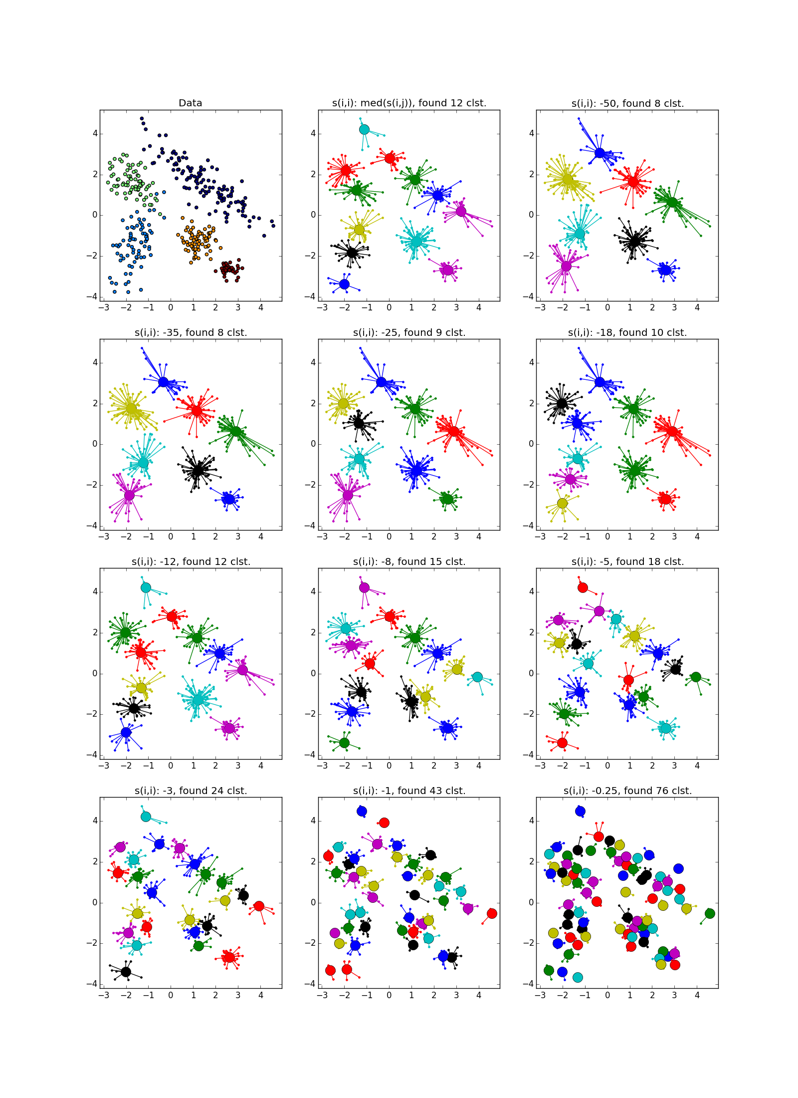
As already mentioned, instead of a predetermined number of clusters, the “self-similarity” parameter is used. s ( k , k ) ; the smaller s ( k , k ) the larger the clusters. There are heuristics for automatic adjustment of the value of this parameter: use the median for all s ( i , k ) for the greater number of clusters; 25 percentile or even at least s ( i , k ) - for less (you still have to customize, ha ha). If the self-similarity value is too small or too large, the algorithm will not produce any useful results at all.
As s ( i , k ) itself suggests to use the negative Euclidean distance between i and j , but no one limits you in choosing. Even in the case of dataset from the vectors of real numbers, you can try a lot of interesting things. In general, the authors argue that the function of similarity is not imposed any special restrictions ; it is not even necessary that the symmetry rule or the triangle rule be fulfilled. But it's worth noting that the more cunning you have s ( i , j ) , the less likely that the algorithm will converge to something interesting.
The sizes of clusters obtained during the proximity propagation vary within rather small limits, and if there are clusters of very different sizes in dataset, the AP can either skip small ones or count large ones for a few. Usually the second situation is less unpleasant - it is fixable. Therefore, the AP often needs to be post-processed - additional clustering of group leaders . Any other method is suitable, additional information about the task can help. It should be remembered that honest lonely standing points stand out their clusters; such emissions need to be filtered before post-processing.
Experiments
Fuh, the wall of the text is over, the wall of pictures has begun. Let's check Affinity propagation on different types of clusters.
Wall of pictures
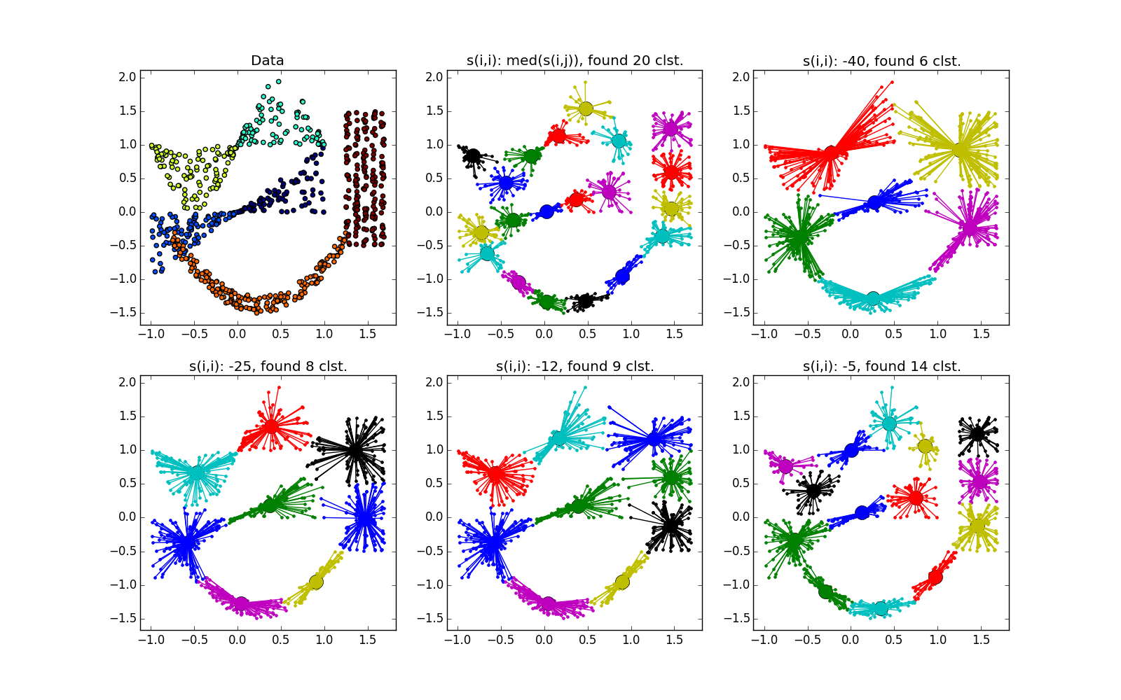
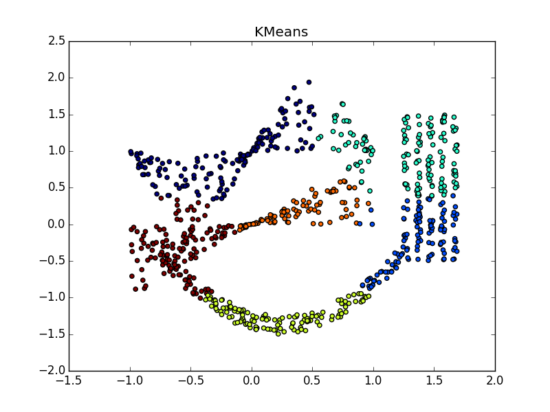
Proximity propagation works well on clusters in the form of folds of dimension less than the dimension of data. AP usually does not select the entire fold, but breaks it into small pieces-subclusters, which then have to be glued together. However, this is not so difficult: with twenty points it is easier than with twenty thousand, plus we have additional information about cluster elongation. This is much better than k-means and many other non-specialized algorithms.
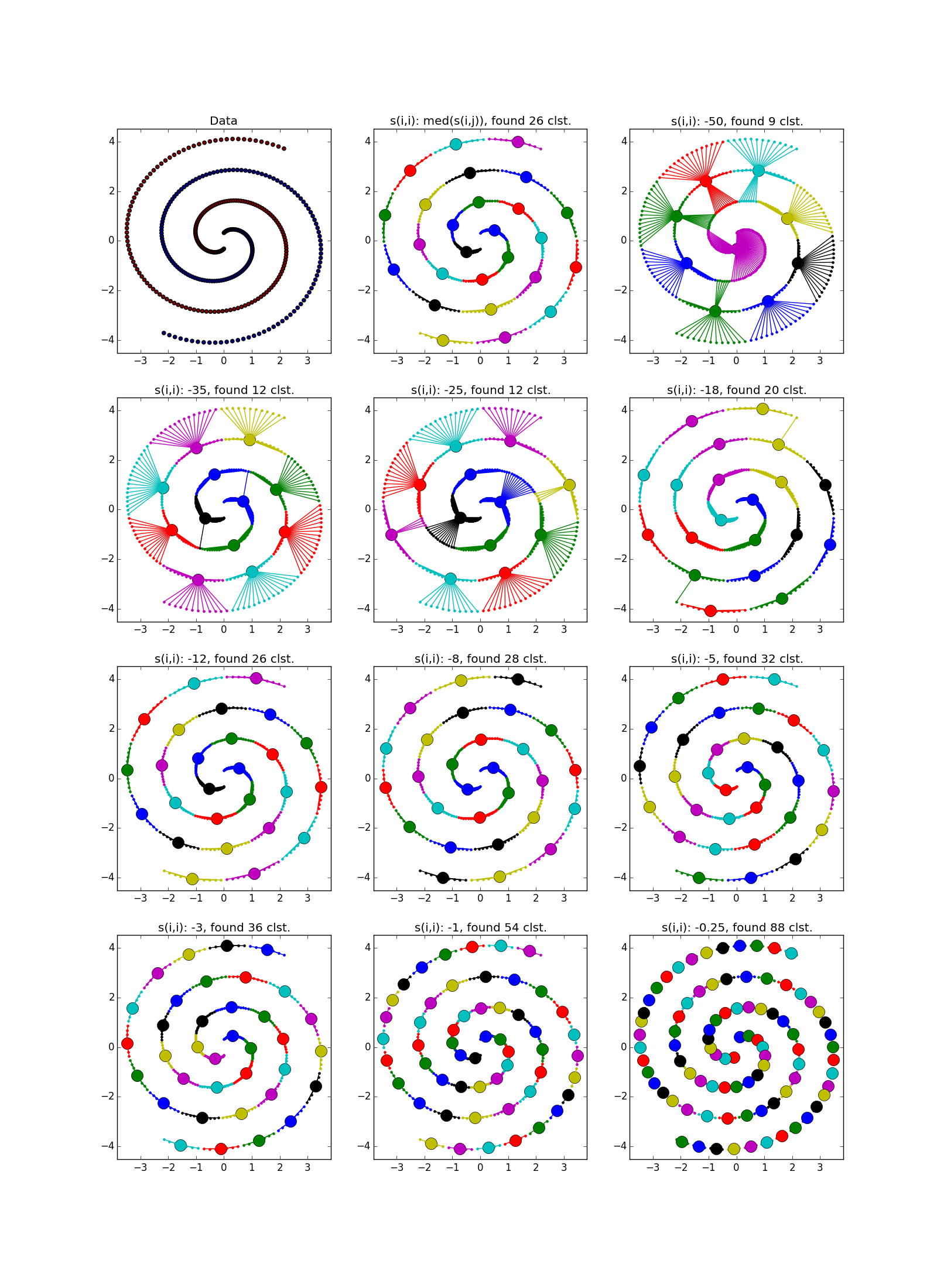
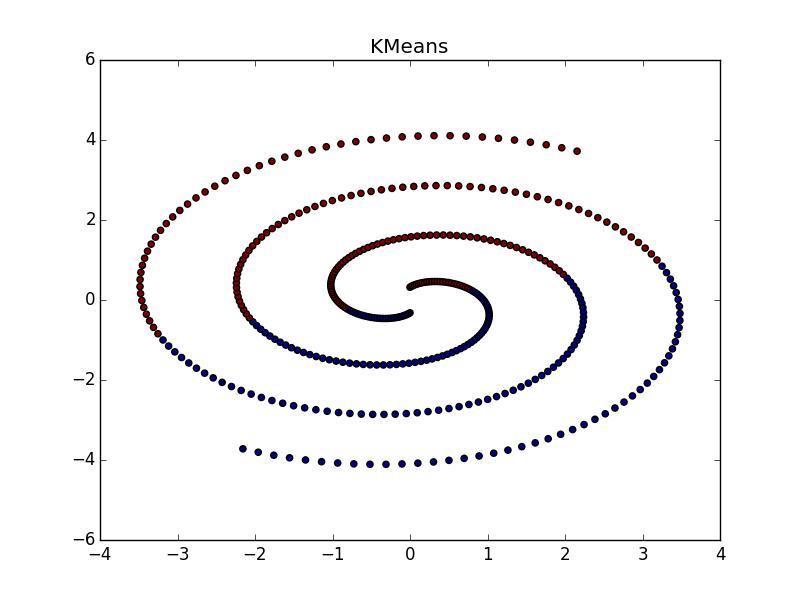
If the fold crosses another clot, the situation is worse, but even so, the AP helps to understand that something interesting is happening in this place.
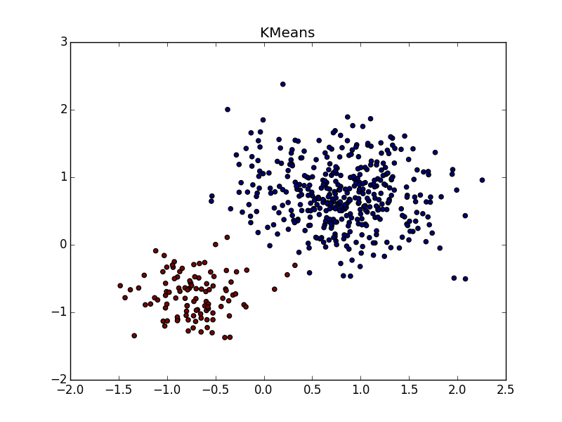
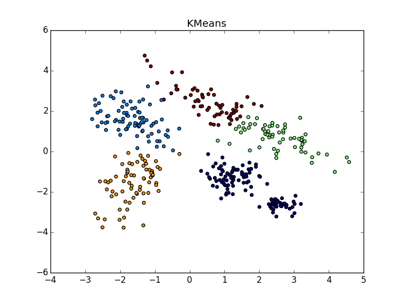
With a good selection of the parameter and the post processing processor, the AP wins even in the case of clusters of different sizes. Pay attention to the picture with s(i,i)=−$ - almost perfect partition, if you combine the clusters from the top to the right.
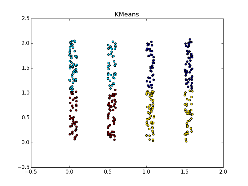
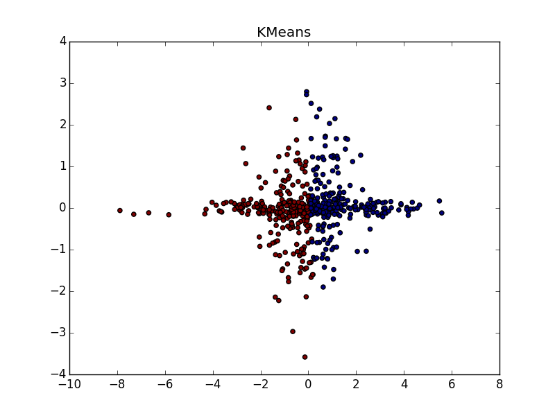
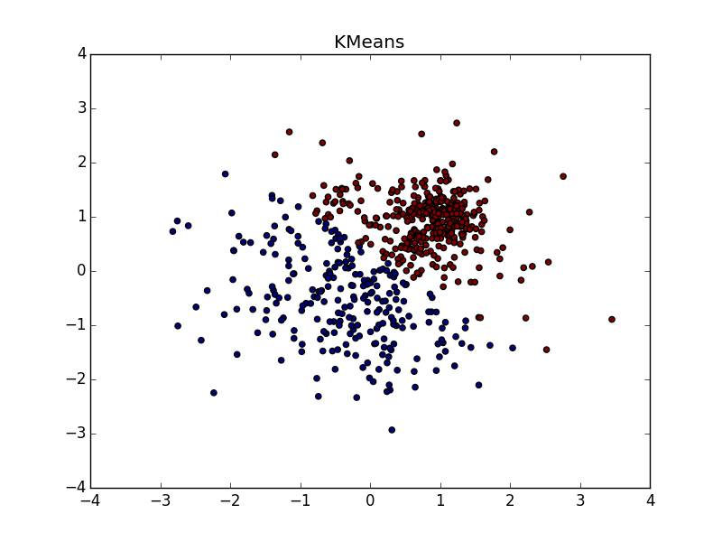
With clusters of the same shape, but different densities for AP and k-means plus or minus parity. In one case, you need to guess well s(i,i) , and in another - k .


With a clot of greater density in another clot, in my opinion, k-means wins a little bit. , , «» , AP .
:
If the fold crosses another clot, the situation is worse, but even so, the AP helps to understand that something interesting is happening in this place.
With a good selection of the parameter and the post processing processor, the AP wins even in the case of clusters of different sizes. Pay attention to the picture with s(i,i)=−$ - almost perfect partition, if you combine the clusters from the top to the right.
With clusters of the same shape, but different densities for AP and k-means plus or minus parity. In one case, you need to guess well s(i,i) , and in another - k .
With a clot of greater density in another clot, in my opinion, k-means wins a little bit. , , «» , AP .
:
Total
Use Affinity propagation when
- You are not very big ( N < 10 5 - 10 6 ) or moderately large, but rarefied (N < 10 6 - 10 7 )
- The proximity function is known in advance.
- You expect to see many clusters of various shapes and a slightly varying number of elements.
- Are you ready to tinker with postprocessing
- The complexity of the elements dataset does not matter
- The proximity function properties do not matter
- The number of clusters does not matter
It is argued that various scientists have successfully used Affinity propagation for
- Image segmentation
- Selection of groups in the genome
- City breaks into accessibility groups
- Clustering Granite Samples
- Netflix Movie Grouping
In all these cases, the result was obtained better than with the help of k-means. Not that this is some kind of awesome result in itself. I don’t know if in all these cases there was a comparison with other algorithms. I plan to do this in future articles. Apparently, in real-life datasets, the ability to distribute proximity helps most of all with clusters of different geometric shapes.
Well, everything seems to be all. Next time we will consider some other algorithm and compare it with the method of proximity propagation. Good luck, Habr!
Source: https://habr.com/ru/post/321216/
All Articles