Study of the qualitative features of the dynamics of mathematical models of nonlinear nonautonomous systems

Yu.A. Bychkov, S.V. Shcherbakov

Investigation of the qualitative features of the dynamics of mathematical models of nonlinear nonautonomous systems using eigenvalues ​​of the Jacobi functional matrix

Formulation of the problem

The task of studying the qualitative features of the dynamics of mathematical models of nonlinear nonautonomous systems with lumped parameters is extremely relevant. The development of the theory of nonlinear phenomena and the obtained applied results generate a variety of methods for solving this problem [1-3].
In the general case, the dynamics of mathematical models of systems of a selected class (hereinafter referred to as “systems”) are described by the following ordinary nonlinear integral-differential equation with non-stationary coefficients:

$$

$$A (D) x (t) = G (D) f (t) + H (x, f, t) \ qquad (1)$$

Where $$$D$ - operator of generalized differentiation with respect to independent variable $$$t$ ; $$$A (D)$ - square, order $$$Lx$ matrix with polynomial from $$$D$ and $$$D ^ {- 1}$ elements where $$$D ^ {- 1}$ - integration operator with a variable upper limit $$$t$ ;
G (D) is a rectangular matrix of size $$$L \ _x \ times L \ _f$ with polynomial from $$$D$ and $$$D ^ {- 1}$ elements; $$$x (t)$ and $$$f (t)$ - matrix columns of the coordinates of the system (the desired solutions) and external influences on it, respectively; $$$H (x, f, t)$ - a column matrix with rows in the form of sums of products whose factors are non-stationary coefficients, as well as classical derivatives of any order and integrals of any multiplicity, starting with zero, from the desired solutions and external influences, in arbitrary fractional rational degrees.

Calculation of the dynamics of nonlinear nonautonomous systems under given pre-initial conditions $$$D ^ nx \ _r (0 ^ -) = D ^ nx \ _r (t \ _0 ^ -)$ , $$$r = 1,2, ..., L \ _x$ , $$$0 ^ - = t ^ - \ _ 0$ , $$$n \ in [0; M-1]$ comes down to finding all existing in a given study interval $$$[t \ _0; T]$ solutions of equation (1) and is associated with a number of algorithmic and mathematical problems. The essence of these problems determines the objective variety of qualitative features of the desired solutions.

In the general case, the nature of the dynamics of the desired solutions of equation (1) is unpredictable, this is due to the dependence of the manifestation forms of the dominant nonlinear and non-stationary properties of the system on the selected initial conditions, the ratio of parameters and the type of its characteristics. In the general case, the indicators of the desired solutions of the equation $$$(1)$ irregular, reducing the dynamics of the system to the so-called deterministic chaos [2-4]. Describing its dynamics, we note that in the desired solutions of the equation $$$(1)$ gaps of the first kind, including differentiable ones, and gaps of the second kind are possible. The specificity of these decisions is that they, as a rule, are associated with "rigidity", i.e. with alternating intervals of fast and slow changes in their dynamic indicators, and within such intervals transitions from local stability to instability and vice versa are possible. A direct consequence of local instability is the effect of “mixing” solutions, which greatly complicates the problem of numerical calculation of the dynamics of a nonlinear nonautonomous system and analysis of its qualitative features [5]. The possible qualitative diversity of the features of the dynamics of a nonlinear nonautonomous system, as a result of the complex synthesis of its coordinate-parametric interconnections, allows only an approximate solution of the equation $$$(1)$ using one or another numerical method [6-8]. There are many numerical methods and their calculation schemes are constantly being improved. However, none of them allows you to establish in a closed form any relationship or pattern between the behavior of the desired solution of the equation $$$(1)$ and information indicators of this equation. The task of identifying such relationships and organizing on their basis a subsequent analysis of the qualitative features and properties of solutions of the equation $$$(1)$ important in both theoretical and applied terms. Its solution means the next step towards understanding the content of cause-effect relationships in nonlinear and non-stationary phenomena.

The article provides a solution to the problem based on the use of the nonlinear nonautonomous system of eigenvalues ​​as information indicators of the dynamics corresponding to its equation $$$(1)$ Jacobi functional matrix and decomposition by such eigenvalues ​​of solutions of this equation. As a computational basis, an analytical-numerical method was used, which according to its computational characteristics corresponds to the task [9, 10]. An illustrative example is provided.

Allocation of information indicators of the dynamics of a nonlinear nonautonomous system

The composition of information indicators of the qualitative features of the desired solutions of the equation $$$(1)$ It is advisable to include those that determine the interaction of the parameters of this equation and the non-stationary indicators of the solutions themselves. In a linear stationary system whose dynamics is described by the equation $$$(1)$ at $$$H (x, f, t) = const$ , such information indicators are the roots $$$\ lambda \ _n, n = 1,2, ..., N$ the following characteristic equation:

$$

$$A (p) = 0 \ qquad (2)$$

Where $$$A (p)$ - determinant of the matrix $$$A (D)$ , when replacing the operator $$$D$ to the operator $$$p$ .

The nature and numerical values ​​of the roots of the equation $$$(2)$ , determine all the features and properties of the dynamics of a linear autonomous system in the transition process, including stability and "rigidity" [1,7,8]. Since external influences unambiguously regulate the nature of the steady state, the dynamics of a linear autonomous system is completely predictable in a semi-infinite time interval.

The directional selection of such information-intensive and fairly simple in determining the dynamics of nonlinear non-autonomous systems is not yet possible. The urgent needs of the practice, however, require already now the selection of indicators of such systems that are available for calculation and are acceptable in terms of the information content. If we follow the same path as for the linear case, then it’s logical to consider the roots as the necessary information indicators $$$\ lambda \ _n, n = 1,2, ..., N$ the equations $$$(2)$ , the formation of which will be associated with the calculation of the determinant $$$A (p)$ matrices $$$A (D)$ selected linear part of the equation $$$(1)$ . The interpretation of the semantic content of the resulting information indicators $$$\ lambda \ _n, n = 1,2, ..., N$ ambiguous because the interrelation of these essentially selected stationary indicators with the qualitative features of the dynamics of a nonlinear nonautonomous system does not lend itself to any meaningful identification, even staged. Also, when in the equation $$$(1)$ matrix $$$A (D)$ zero or highlighted by non-linear part $$$H (x, f, t)$ this equation, then the roots of the equation $$$(2)$ generally absent or their existence, and therefore the content, is conditionally subjective [9].
Thus, the target attribute of the selection of acceptable information indicators of the dynamics of a nonlinear non-autonomous system is the condition of their existence and the mathematical relationship with the numerical indicators of the desired solution of the equation $$$(1)$ . This condition can be satisfied if in the equation $$$(1)$ linear part matrix $$$A (D)$ in a certain way to select or supplement at the expense of the matrix $$$H (x, f, t)$ nonlinear part [9,10]. This selection or addition of the matrix $$$A (D)$ due to the matrix $$$H (x, f, t)$ perhaps in an ambiguous way. All transformations performed during this process must be equivalent, as a result of which the dynamics of the system will remain unchanged. As a result of the selection or addition of the matrix $$$A (D)$ due to the matrix $$$H (x, f, t)$ the necessary mathematical relationship of the roots will be achieved $$$\ lambda \ _n, n = 1,2, ..., N$ the equations $$$(2)$ with the numerical values ​​of the desired solutions of the equation $$$(1)$ at discrete points in time, determined by the step of numerical calculation of the dynamics of the system. Thus, as a result of these transformations of the equation $$$(1)$ the roots $$$\ lambda \ _n, n = 1,2, ..., N$ the equations $$$(2)$ will acquire a functional dependence on time, both in relation to numerical indicators and qualitative characteristics.

Nonstationary root properties $$$\ lambda \ _n, n = 1,2, ..., N$ the equations $$$(2)$ in the absence of a target criterion for the implementation of the corresponding matrix transformations $$$A (D)$ leading to the appearance of such properties cannot by themselves guarantee the necessary informative characteristics of these roots. The desired study of the qualitative features of the dynamics of nonlinear objects dictates the choice as the target criterion for the formation or transformation of an existing matrix $$$A (D)$ the equations $$$(1)$ the condition of its coincidence with the Jacobi functional matrix corresponding to this equation [4–8]. The algorithm for solving this problem is described in [10]. As a result of the formation or transformation of the matrix $$$A (D)$ due to the matrix $$$H (x, f, t)$ to the Jacobi functional matrix of non-stationary roots $$$\ lambda \ _n, n = 1,2, ..., N$ the equations $$$(2)$ acquire the status of eigenvalues ​​of the Jacobi matrix.

Nonstationary eigenvalues $$$\ lambda \ _n, n = 1,2, ..., N$ Jacobi functional matrix of the equation $$$(1)$ at discrete points in time, determined by the step of its numerical solution, have a certain well-known semantic content [4-8]. Being a local characteristic of the dynamics of a nonlinear nonautonomous system, they in the infinitely small neighborhood of a point corresponding to a discrete point in time t characterize the stability and rate of change of dynamic indicators of solutions of its dynamic equation $$$(1)$ . In the neighborhood of the singular points of the equation $$$(1)$ own numbers $$$\ lambda \ _n, n = 1,2, ..., N$ Jacobi’s functional matrix allows one to isolate areas of attraction and repulsion of phase trajectories on the phase plane, thus giving a forecast for the limiting states of existing solutions of this equation [6–8]. Eigenvalues ​​corresponding to discrete points in time $$$\ lambda \ _n, n = 1,2, ..., N$ the Jacobi functional matrix, characterizing and determining the qualitative features and properties of the dynamics of nonlinear nonautonomous systems, determine the relevance of the task of identifying mathematical features and information indicators of such a relationship. The solution of this problem is associated with the establishment of a mathematical relationship between the selected non-stationary information indicators $$$\ lambda \ _n, n = 1,2, ..., N$ the dynamics of a nonlinear nonautonomous system and the parameters of the calculation scheme of the numerical method used to calculate this dynamics. A prerequisite for achieving this goal is the presence in the calculation scheme of the selected method of the corresponding analytical part. The computational algorithm of this analytical part of the method must be consistent with the peculiarities of calculating the eigenvalues ​​of the Jacobi functional matrix, and also provide a mathematical relationship between these numbers and the dynamic coordinates of the coordinates of a nonlinear non-autonomous system. The one-step analytical-numerical method of variable order [9, 10] fully meets the formulated requirements.

Analytical-numerical method for calculating the dynamics of nonlinear nonautonomous systems

The motivation for the formation of the analytical-numerical method was the desire to unify the solution of the equation $$$(1)$ using only identical transformations. Hence the description of the desired solutions by Taylor series and the subsequent application of the Laplace integral for the algebraization of the problem.
Analytical-numerical method for calculating the dynamics of the selected equation $$$(1)$ class of systems in a given study interval $$$[t \ _0; T]$ consists of two parts: analytical and numerical.
The analytical part of the method is based on apparatuses of generalized functions, the Laplace transform, and function-power series. The procedure of the analytical part precedes the execution of each successive calculation step and reduces to the following. First, by expanding the functions describing external actions and non-stationary parameters of the system, into their corresponding power series, and also formally describing the regular components of the desired solutions that are included in the matrix $$$H (x, f, t)$ the equations $$$(1)$ corresponding to their power series, we transform the right-hand side of this equation into a matrix-column, the rows of which are now power series. The coefficients of these power series are generally unknown, since they are expressed in terms of known coefficients of power series for external influences and non-stationary parameters of the system, and unknown coefficients of power series for the regular components of some of the desired solutions. The performed operation gives the original equation $$$(1)$ to the form required for the subsequent application of the integral Laplace transform. Transforming Laplace's Reformed Equation $$$(1)$ and solving the resulting algebraic equation according to Cramer’s rule, for the image $$$X \ _l (p)$ the desired solution $$$x \ _l (t), l \ in [1, L \ _x]$ we get the following expression:

$$

$$X \ _l (p) = \ frac {B ^ l \ _l (p)} {A (p)} = \ frac {\ sum \ limits \ _ {i = 0} ^ \ infty B ^ l \ _ { l.N + J \ _l-i} p ^ {N + J \ _l-i}} {\ sum \ limits \ _ {i = 0} ^ NA \ _ {i} p ^ i}, \ qquad (3 )$$

Where $$$N \ in \ mathbb N; J \ _l \ in \ mathbb Z$

Fractional rational function, described by expression (3), in the general case, when $$$J \ _l \ geq 0$ is incorrect and allows its presentation as a sum of a whole rational $$$X \ _l ^ - (p)$ and correct fractional rational $$$X \ _l ^ + (p)$ functions. The subsequent decomposition of the correct fractional rational function $$$X \ _l ^ + (p)$ the Laurent series in the neighborhood of an infinitely remote point transforms the expression $$$(3)$ in the following way:

$$

$$X \ _ {l} (p) = X \ _ {l} ^ {-} (p) + X \ _ {l} ^ {+} (p) = \ \ sum \ _ {j = 0} ^ {-J \ _ {l}} S \ _ {lj} p ^ {- j} + \ frac {\ sum \ limits \ _ {i = 1} ^ {\ infty} B \ _ {lN-i} p ^ {Ni}} {\ sum \ limits \ _ {i = 0} ^ {N} A \ _ {i} p ^ {i}} = \\\\ = \ sum \ _ {j = 0} ^ { -J \ _ {l}} S \ _ {lj} \; p ^ {- j} \; + \; \ frac {\ sum \ limits \ _ {i = 0} ^ {\ infty} B \ _ {l.N-i-1} \; \; p ^ {N-i}} {\ sum \ limits \ _ {i = 0} ^ {N} A \ _ {i} \; p ^ {i}} \; \; \ frac {1} {p} = \\\\ = \ sum \ _ {j = 0} ^ {- J \ _ {l}} S \ _ {l.j} \; p ^ {- j} \; + \; \ sum \ _ {i = 0} ^ {\ infty} R \ _ {l.i} \; p ^ {- (i + 1)}. \ qquad (4)$$

Coefficients $$$S \ _ {l.j}$ , $$$B \ _ {l.N-i}$ , $$$R \ _ {l.i}$ included in the expression $$$(4)$ , taking into account the notation of expression $$$(3)$ , calculated by the following formulas [9,10]:

$$

$$S \ _ {l. \; -J \ _ {l}} = \ frac {B ^ l \ _ {l.N + J \ _ {l}}} {A \ _ {N \; }};$$

$$

$$S \ _ {l. \; -J \ _ {l} + j} = \ frac {B ^ l \ _ {l.N + J \ _ {l} + j} - \ sum \ limits \ _ {k = 0} ^ {j-1 } S \ _ {l.-J \ _ {l} + k} \; A \ _ {N-j + k \; }} {A \ _ {N}}$$

,
Where $$$j = 1,2, ..., J \ _ {l};$

$$

$$B \ _ {l.N-i} = B ^ l \ _ {l.N-i} - \; \ sum \ _ {k = 0} ^ {N-i} S \ _ {l.-N + i + k} \; A \ _ {k}$$

Where $$$i = 1,2, ...; S \ _ {l.-r} = 0,$ if a $$$r> J \ _l;$

$$

$$\ begin {align} & {R \ _ {l.0} = \ frac {B \ _ {lN-1}} {A \ _ {N}};} \\ & {R \ _ {li} = \ frac {B \ _ {lN-1-i} - \ sum \ limits \ _ {k = 0} ^ {i-1} R \ _ {lk} \; A \ _ {N-i + k}} {A \ _ {N}},} \ end {align} \ qquad (5)$$

Where $$$i = 1,2, ...$

The terms of the sum on the right side of the last equation $$$(4)$ form respectively the main and the right parts of the Laurent series for the image $$$X \ _ {l} (p)$ the desired solution $$$x \ _ {l} (t), l \ in [1; L \ _ {x}]$ in the neighborhood of an infinitely distant point. Original for the image $$$X \ _ {l} (p)$ serves as a generalized function $$$x \ _ {l} (t), l \ in [1; \; L \ _ {x}]$ containing singular $$$x \ _ {l} ^ {-} (t)$ and regular $$$x \ _ {l} ^ {+} (t)$ components.
So, after performing the analytical part of the method for the desired solution $$$x \ _ {l} (t), l \ in [1; \; L \ _ {x}]$ the equations $$$(1)$ we get the following description:

$$

$$x \ _ {l} (t) = x \ _ {l} ^ {-} (t) + x \ _ {l} ^ {+} (t) = \ sum \ _ {j = 0} ^ { -J \ _ {l}} S \ _ {lj} \; {\ rm \ delta} \ _ {j} (t) + \ sum \ _ {i = 0} ^ {\ infty} R \ _ {l.i} \; t ^ {i} / i! \; , \ qquad (6)$$

Where $$${\ rm \ delta} \ _ {j} (t)$ - impulse functions from zero to$$ $ inline $ -J \ _ {l} $ inline $ -th order inclusive, defined in the starting point for the considered interval of calculation; $$$S \ _ {l.j}$ - weight coefficients of impulse functions; $$$R \ _ {l.i}$ - coefficients of decomposition of the regular component of the solution $$$x \ _ {l} ^ {+} (t)$ in the power series in the right neighborhood of the initial for the considered interval of calculation the point with the abscissa $$$t = 0 ^ {+}$ [9,10].

The resulting form $$$(6)$ descriptions of the desired solution $$$x \ _ {l} (t), l \ in [1; \; L \ _ {x}]$ reflects a number of fundamental points related to the analysis of the qualitative features of the dynamics of nonlinear nonautonomous systems. The use of the integral Laplace transform allows at the point corresponding to the beginning of the current calculation interval to make the correct transition from the known initial conditions to the initial conditions to be determined and to select the required solutions in the desired solutions. $$$(1)$ breaks of the first kind, if they exist. Presence in the description $$$(6)$ singular component $$$x \ _ {l} ^ {-} (t)$ indicates the possibility of distinguishing existing differentiated discontinuities of the first kind. Note that the singular component of the solution $$$x \ _ {l} ^ {-} (t)$ if it exists, it is available for determination at a discrete point in time, corresponding to the beginning of the current calculation step, in the analytical part of the method.
')
Regular part of the solution $$$x \ _ {l} ^ {+} (t)$ as follows from the description $$$(6)$ , is represented by a power series and for its calculation in the current interval of calculation is the numerical part of the method. The basis of the numerical part of the method is the discretization of the independent variable $$$t$ . In the current calculation interval $$${\ rm \; [} t \ _ {k-1}; \; t \ _ {k}] {\ rm \; }, {\ rm \; } t \ _ {k} = t \ _ {k-1} + h \ _ {k}$ implementation of the numerical part of the method begins with the selection of the appropriate step size $$$h = h \ _ {k}$ . This choice is governed by the following equality [9,10]:

$$

$$h = q {\ rm \ tau,} \ qquad (7)$$

Where $$$0 <q <1.$
Limit value $$$\ tau$ the length of the current calculation step $$$h$ equality $$$(7)$ , is the result of convergence research in the current interval of calculating the numerical majorant power series for regular components $$$x \ _ {r} ^ {+} \ left (t \ right)$ sought solutions $$$x \ _ {r} (t) {r} = 1,2, {\ dots}, L \ _ {x}$ . The length of the current calculation step $$$h = h \ _ {k}$ chosen according to equality $$$(7)$ , is such that it ensures the fulfillment of a number of significant conditions for the analysis of the qualitative features of the dynamics of nonlinear nonautonomous systems.

First, in the current calculation interval $$${\ rm \; [} t \ _ {k-1}; \; t \ _ {k}] {\ rm \; }, {\ rm \; } t \ _ {k} = t \ _ {k-1} + h \ _ {k}$ all power series for regular components of solutions $$$x \ _ {r} ^ {+} \ left (t \ right)$ converge to the functions laid out in them, turning into Taylor series. This indicates the existence of the desired solutions in the considered time interval. $$$x \ _ {r} ^ {+} \ left (t \ right)$ , giving the entire computational procedure a logical meaning and practical feasibility.

Secondly, selected according to equality $$$(7)$ step size calculation $$$h = h \ _ {k}$ provides numerical stability of the calculation procedure at a discrete point in time $$$t = t \ _ {k}$ approximate value $$$x \ _ {l} ^ {+} (t \ _ {k}; {\ rm \;} I \ _ {l})$ regular component $$$x \ _ {l} ^ {+} (t)$ the desired solution $$$x \ _ {l} (t), l \ in [1; \; L \ _ {x}]$ . Calculation of the approximate value of the solution $$$x \ _ {l} ^ {+} (t \ _ {k}; {\ rm \;} I \ _ {l})$ associated with limiting the taylor series to the regular component of the solution $$$x \ _ {l} ^ {+} (t)$ partial sum of his first $$$I \ _ {l}$ members. The residual term of the series arising in this case, forming a local calculation error, is always limited and available for upper estimates using the formulas given in [9, 10].

Third, step length $$$h = h \ _ {k}$ always corresponds to the rate of change of the regular components $$$x \ _ {r} ^ {+} \ left (t \ right)$ desired solutions. This result is provided by the organization of the study of convergence of power series for regular components of solutions $$$x \ _ {r} ^ {+} \ left (t \ right)$ by considering the corresponding numeric majorant. Their members are formed by all possible combinations of the coefficients of these power series, which determine the values ​​of the derivatives of final orders from these decision components at a discrete point in time $$$t = t \ _ {k-1}$ .

Fourth, corresponding to equality $$$(7)$ step size calculation $$$h = h \ _ {k}$ such that allows you to organize a procedure for the upper assessment $$$| \ Delta x \ _ {l} ^ {+} (t; {\ rm \;} I \ _ {l}) {\ rm |} t = t \ _ {k}$ absolute full error of calculation of the approximate value $$$x \ _ {l} ^ {+} (t \ _ {k}; {\ rm \;} I \ _ {l})$ regular component $$$x \ _ {l} ^ {+} (t)$ the desired solution $$$x \ _ {l} (t), l \ in [1; \; L \ _ {x}]$ . By complete calculation error, we mean the error accumulated after performing two or more calculation steps, at each of which a local calculation error occurs.

So, choosing according to equality $$$(7)$ the value of the current calculation step $$$h = h \ _ {k}$ and limiting the taylor series to the regular component of the solution $$$x \ _ {l} ^ {+} (t)$ partial sum of his first $$$I \ _ {l}$ members, we calculate the approximate value $$$x \ _ {l} ^ {+} (t \ _ {k}; {\ rm \;} I \ _ {l}), t \ _ {k} = t \ _ {k-1} + h \ _ {k}$ this component of the solution. Then, appreciating the current step $$$h = h \ _ {k}$ local calculation error, we calculate the upper estimate $$$| \ Delta x \ _ {l} ^ {+} (t; {\ rm \;} I \ _ {l}) {\ rm |}, t = t \ _ {k}$ full error of calculation. Numerical results obtained in this way allow at a discrete point in time $$$t = t \ _ {k}$ select a one-dimensional interval on the ordinate axis that contains an unknown exact value $$$x \ _ {l} ^ {+} (t \ _ {k})$ regular component $$$x \ _ {l} ^ {+} (t)$ the desired solution. In the accepted notation, this interval is at a discrete point in time. $$$t = t \ _ {k}$ describes the following double inequality:

$$

$$x \ _ {l} ^ {+} (t \ _ {k}; {\ rm \;} I \ _ {l}) \; - | \ Delta x \ _ {l} ^ {+} (t \ _ {k}; {\ rm \;} I \ _ {l}) {\ rm |} \ le x \ _ {l} ^ { +} (t \ _ {k}) \ le x \ _ {l} ^ {+} (t \ _ {k}; {\ rm \;} I \ _ {l}) + | \ Delta x \ _ {l} ^ {+} (t \ _ {k}; {\ rm \;} I \ _ {l}) {\ rm |}. \ qquad (8)$$

Equality $$$(6)$ and double inequality $$$(8)$ describe the results of the computational procedure of the analytical-numerical method at the current calculation step $$$h = h \ _ {k}$ . To perform the next calculation step in the specified study interval $$${\ rm \; [} t \ _ {0}; \; T]$ the axis of ordinates is transferred to the right by the value $$$h \ _ {k}$ . After that, choosing from double inequalities $$$(8)$ at $$$l = r, r = 1,2, {\ dots}, L \ _ {x}$ any approximate values ​​of pre-initial conditions, we repeat the described procedures of the analytical and numerical parts of the method.

### ** Establishing the relationship of information indicators of the dynamics of a nonlinear nonautonomous system and parameters of the design scheme of an analytical-numerical method. **
Expression analysis $$$(3)$ taking into account the equation $$$(2)$ shows that the achievement of this goal is possible by establishing a mathematical relationship between the poles $$${\ rm \; } \ lambda \ _ {n}, {\ rm \; } n = 1,2, ..., N {\ rm \; }$ Images $$$X \ _ {l} (p)$ the desired solution $$$x \ _ {l} (t), l \ in [1; \; L \ _ {x}]$ and dynamic indicators of the quality features and properties of the regular component $$$x \ _ {l} ^ {+} (t)$ this decision. As such dynamic indicators of the regular component of the solution $$$x \ _ {l} ^ {+} (t), l \ in [1; \; L \ _ {x}]$ reasonably motivated consideration of the coefficients $$$R \ _ {l.i}$ included in the description $$$(6)$ power series. Calculation of coefficients $$$R \ _ {l.i}$ perform in the analytical part of the method using recurrent formulas $$$(5)$ . Transforming these formulas using matrix analysis leads to their new form of record, which explicitly establishes the necessary mathematical relationship between coefficients. $$$R \ _ {l.i}$ regular component of the solution $$$x \ _ {l} ^ {+} (t)$ and poles $$${\ rm \; } \ lambda \ _ {n}, {\ rm \; } n = 1,2, ..., N {\ rm \; }$ Images $$$X \ _ {l} ^ {+} (p)$ this component. New formulas for calculating coefficients $$$R \ _ {l.i}$ are given in [8]. So, for example, when all the poles $$${\ rm \; } \ lambda \ _ {n}, {\ rm \; } n = 1,2, ..., N {\ rm \; }$ Images $$$X \ _ {l} ^ {+} (p)$ simple formula for calculating coefficients $$$R \ _ {l.i}$ has the following form [8]:

$$

$$R \ _ {l.i} = \ sum \ _ {n = 1} ^ {N} r \ _ {l.n} \; \ lambda \ _ {n} ^ {i} \; , \; \; i \ in \ ge \ left | {\ bf Z} \ right |. \ qquad (9)$$

Coefficients $$$r \ _ {l.n}$ in this case, we calculate by the formula:

$$

$$r \ _ {l.n} = \ frac {\ sum \ limits \ _ {m = 1} ^ {i} B \ _ {l.N-1-m} ^ {\ *} \; \ lambda \ _ {n} ^ {- m} \; } {N + \ sum \ limits \ _ {m = 1} ^ {N-1} (N-m) \; A \ _ {Nm} ^ {\ *} \; \ lambda \ _ {n} ^ {- m}}. \ qquad (10)$$

Coefficients $$$B \ _ {l.N-1-m} ^ {\ *}, \; \; m \ in \ left | {\ bf Z} \ right |$ and $$$A \ _ {r} ^ {\ *}, \; \; r = 1,2, ..., N-1$ in the formula $$$(10)$ associated with coefficients $$$B \ _ {l.N-1-m} ^ {} \; , \; \; A \ _ {r}$ included in the expression $$$(4)$ , by the following relations:

$$

$$\ begin {align} & {B \ _ {l.N-1-m} ^ {\ *} = \ frac {B \ _ {l.N-1-m}} {A \ _ {N}} \; ;} \\\\ & {A \ _ {r} ^ {\ *} = \ frac {-A \ _ {r}} {A \ _ {N}} \; .} \ end {align}$$

Formula $$$(9)$ allows you to write the description $$$(6)$ power series for the regular component $$$x \ _ {l} ^ {+} (t)$ the required solution in this case in the following new form [8]:

$$

$$x \ _ {l} ^ {+} (t) = \ sum \ _ {i = 0} ^ {\ infty} \ frac {R \ _ {l.i} \; t \ _ {} ^ {i}} {i!} = \ sum \ _ {i = 0} ^ {\ infty} \ sum \ _ {n = 1} ^ {N \ _ {m}} \ frac { R \ _ {li} ^ {[n]} t \ _ {} ^ {i}} {i!}, \ Qquad (11)$$

Where $$$N \ _ {m}$ - the number, in this case simple, of the image poles $$$X \ _ {l} ^ {+} (p)$ .

Formed description $$$(11)$ causes for the regular component $$$x \ _ {l} ^ {+} (t)$ the desired solution $$$x \ _ {l} (t), l \ in [1; \; L \ _ {x}]$ following equivalent representation:

$$

$$x \ _ {l} ^ {+} (t) = \ sum \ _ {n = 1} ^ {N \ _ {m}} x \ _ {l} ^ {[n]} (t) \; . \ qquad (12)$$

Components $$$x \ _ {l} ^ {[n]}$ they have the following description:

$$

$$x \ _ {l} ^ {[n]} (t) = \ sum \ _ {i = 0} ^ {\ infty} \ frac {R \ _ {l.i} ^ {[n]} \; t \ _ {} ^ {i}} {i!}. \ qquad (13)$$

interrelated equality system $$$(11) - (13)$ Is the result of the directed transformation of the incoming equality $$$(6)$ source description of the regular component of the solution $$$x \ _ {l} ^ {+} (t)$ . According to it, at each calculation step, this component of the solution can be decomposed by poles $$${\ rm \; } \ lambda \ _ {n}, {\ rm \; } n = 1,2, ..., N {\ rm \; }$ her images $$$X \ _ {l} ^ {+} (p)$ . Decomposition, as one would expect, is not absolute, because through recurrently calculated coefficients $$$B \ _ {l.N-1-m} ^ {\ *}, \; \; m \ in \ left | {\ bf Z} \ right |$ included in the formula $$$(10)$ , for a nonlinear nonstationary system, the relationship between all elements that always dominates in the formation of its dynamics is always preserved $$$(13)$ representation $$$(12)$ . Decomposition of the regular component $$$x \ _ {l} ^ {+} (t)$ the desired solution $$$x \ _ {l} (t), l \ in [1; \; L \ _ {x}]$ described by a system of equalities $$$(11) - (13)$ , was successfully tested when solving a number of special problems related to the formalization of the procedure for studying the existence and uniqueness of a solution, choosing a calculation step, as well as optimizing the computational costs associated with estimating the absolute local error of such a calculation [9].

Summing up, we formulate the following algorithm for studying the qualitative features of the dynamics of nonlinear nonautonomous systems. First, perform the equivalent transformation of the original equation $$$(1)$ system dynamics to mind when the matrix $$$A (D)$ coincides with the Jacobi functional matrix, then the poles $$${\ rm \; } \ lambda \ _ {n}, {\ rm \; } n = 1,2, ..., N {\ rm \; }$ Images $$$X \ _ {l} ^ {+} (p)$ match the eigenvalues ​​of this matrix. Subsequent decomposition of the regular component of the solution $$$x \ _ {l} ^ {+} (t)$ on these numbers will provide the possibility of organizing a design scheme for the necessary research. In the role of non-stationary information indicators of the qualitative features of the system dynamics, we consider the functions describing the change in a given study interval. $$${\ rm \; [} t \ _ {0}; \; T]$ proper numbers $$${\ rm \; } \ lambda \ _ {n}, {\ rm \; } n = 1,2, ..., N {\ rm \; }$ Jacobi functional matrix and elements $$$(13)$ decomposition $$$(12)$ regular component of the solution $$$x \ _ {l} ^ {+} (t)$ . The proposed decomposition scheme for the desired solutions of the equation $$$(1)$ over eigenvalues ​​of the Jacobi functional matrix corresponding to this equation is extraordinary in and of itself. This determines the novelty of the expected results, their interpretation and subsequent application prospects. We will designate only some of them, since the completeness of judgments about such a problem is a matter of time.

Signs of real parts of non-stationary eigenvalues $$${\ rm \; } \ lambda \ _ {n}, {\ rm \; } n = 1,2, ..., N {\ rm \; }$ Jacobi functional matrix at each discrete point in time $$$t = t \ _ {k}$ determine the possibility of identifying the boundaries of the intervals of stability and instability in relation to each of the elements $$$(13)$ decomposition $$$(12)$ . Such information is primary to identify causal relationships between the sustainability conditions of the regular component of the solution. $$$x \ _ {l} ^ {+} (t), l \ in [1; \; L \ _ {x}]$ and similar conditions for the elements themselves $$$(13)$ this component. Conditions of stability or instability of the regular component $$$x \ _ {l} ^ {+} (t)$ the desired solution $$$x \ _ {l} (t)$ this will be a consequence of the existence of non-stationary eigenvalues $$${\ rm \; } \ lambda \ _ {n}, {\ rm \; } n = 1,2, ..., N {\ rm \; }$ Jacobi's functional matrix of one or several dominant ones, and also on the features of the interaction of these dominant numbers in the study interval, including the variation of their nature.

Dynamic indicators of decomposition elements $$$(13)$ in conjunction with nonstationary eigenvalues $$${\ rm \; } \ lambda \ _ {n}, {\ rm \; } n = 1,2, ..., N {\ rm \; }$ Jacobi functional matrix determine the initial position for a different interpretation of the result of the calculation of the dynamics of a nonlinear non-autonomous system described by double inequality $$$(8)$ . Mathematical interrelation and correlation in the course of calculation of indicators of double inequality $$$(8)$ and double inequalities like inequalities $$$(8)$ but for corresponding elements of decomposition $$$(13)$ with the irregularity of the dynamic properties of the system, serve as the basis for the selection of characteristic ratios and combinations between the elements of the decomposition $$$(13)$ for which the desired solutions of the equation $$$(1)$ most sensitive to changes in parameters and external influences of the system. The analysis of the results obtained in this case makes it possible to isolate the conditions that determine the occurrence of bifurcation, or the ranges of initial conditions leading to the “mixing” of phase trajectories [5].

Qualitative features and characteristic properties of the functions describing the change in a given study interval $$${\ rm \; [} t \ _ {0}; \; T]$ nonstationary eigenvalues $$${\ rm \; } \ lambda \ _ {n}, {\ rm \; } n = 1,2, ..., N {\ rm \; }$ Jacobi’s functional matrix, including the continuity and monotony of these functions, the presence of extremum points, the variability of the nature of such numbers and the sign of their real parts, undoubtedly reflect the essence of the internal causal relationships of the equation $$$(1)$ . As a result, the features and properties of these functions are highly adaptive indicators of the qualitative features of the dynamics of a nonlinear nonautonomous system. The diversity of the content spectrum and the variability of the manifestations of such indicators of the system’s dynamics are still to be determined and this constitutes an independent task, the solution of which may serve as a starting point for a more complete understanding of the complex and ambiguous behavior of the nonlinear object of study. Separating and classifying the relationships between these functional indicators and the qualitative features of a nonlinear nonautonomous system should lead to the emergence of new computational algorithms for analyzing nonlinear and non-stationary phenomena, including determining the conditions for the existence of regular dynamics or the transition to deterministic chaos [2-5].

Conclusion

Described by the system of equalities $$$(11) - (13)$ decomposition of the regular components of the desired solutions of the equation $$$(1)$ introduces into consideration and activates as an independent computational toolkit of analysis of the dynamics of a nonlinear nonautonomous system, the eigenvalues ​​of the Jacobi functional matrix. They generate features and dynamic properties of decomposition elements. $$$(13)$ . As shown in the following example, the analysis of such features and dynamic properties of the decomposition elements $$$(13)$ leads to the selection of new conditions for the existence of one of the characteristic properties of nonlinear dynamics - "stiffness" [1,4,5].

Summarizing what has been said, we note that there are many variants of manifestations of qualitative features and characteristic properties of nonlinear dynamics, they are diverse in terms of the conditions of occurrence and the forms of manifestations. Irregularity, as a property of such dynamics, is rather the norm than the exception [2]. The reasons for such a complex and unpredictable dynamics of a nonlinear non-autonomous system are laid down in the structure and composition of the internal parametric relationships of the dynamic equation. $$$(1)$ . One of the components of the complex indicator of such interrelations is undoubtedly eigenvalues $$${\ rm \; } \ lambda \ _ {n}, {\ rm \; } n = 1,2, ..., N {\ rm \; }$ Jacobi functional matrix. Analysis of the qualitative features of the dynamics of a nonlinear nonautonomous system based on the decomposition of the desired solutions of its dynamic equation $$$(1)$ into components, each of which corresponds to one of the eigenvalues $$${\ rm \; } \ lambda \ _ {n}, {\ rm \; } n = 1,2, ..., N {\ rm \; }$ Jacobi’s functional matrix, while maintaining the logical and mathematical relationship between these components, reflects the essence of the proposed approach to conducting relevant research and a new methodology.

Example
Investigation of the qualitative features of the dynamics of a non-linear autonomous system based on the decomposition of solutions of its dynamic equation by eigenvalues ​​of the Jacobi functional matrix corresponding to this equation
In the shape of $$$(1)$ the dynamic equation of the considered nonlinear autonomous system has the following form:

$$$$ display $$ \ begin {equation} \ left \ | \ begin {array} {cc} {a \ _ {1.1} ^ {[1]} D + a \ _ {1.1} ^ {[0]}} & {0} \\\\ {a \ _ {2.1 } ^ {[0]}} & {a \ _ {2.2} ^ {[1]} D} \ end {array} \, \ right \ | \, \ left \ | \, \ begin {array} {c} {x \ _ {1} (t)} \\\\ {x \ _2 (t)} \ end {array} \ right \ | = \ left \ | \ begin {array} {c} {g \ _ {1.1} ^ {[0]}} \\\\ {0} \ end {array} \ right \ | f (t) + \ left \ | \ begin { array} {c} {h \ _ {1.1} x \ _ {1} ^ 2 (t) x \ _2 (t)} \\\\ {h \ _ {2.1} x \ _ {1} ^ {2 } (t) x \ _ {2} (t)} \ end {array} \ right \ |, \ qquad (14) \ end {equation} $$ display $$

Where $$$a \ _ {1.1} ^ {\ left [1 \ right]} = a \ _ {2.2} ^ {\ left [1 \ right]} = h \ _ {{\ kern 1pt} 1.1} = 1; h \ _ {{\ kern 1pt} 2.1} = -1; f \ left (t \ right) = {\ rm \ delta} \ _ {{\ kern 1pt} 1} \ left (t \ right); g { \ kern 1pt} \ _ {1.1} ^ {\ left [0 \ right]} = \ textit {A}; a {\ kern 1pt} \ _ {1.1} ^ {\ left [0 \ right]} = B + 1; a {\ kern 1pt} \ _ {2.1} ^ {\ left [0 \ right]} = -B.$
After substitution of the values ​​of the parameters specified in the explication to the equation $$$(14)$ , obtained the following unified form of this equation:

$$$$ display $$ \ begin {equation} \ left \ | \ begin {array} {cc} {D {\ rm + B + 1}} & {0} \\\\ {-B} & {D} \ end {array} \ right \ | \, \ left \ | \ begin {array} {c} {x \ _ {1} (t)} \\\\ {x \ _ {2} (t)} \ end {array} \ right \ | = \ left \ | \ begin {array} {c} {A} \\\\ {0} \ end {array} \ right \ | \ delta \ _ {1} (t) + \ left \ | \ begin {array} {c} {x \ _ {1} (t) ^ {2} x \ _ {2} (t)} \\\\ {-x \ _ {1} (t) ^ {2 } x \ _ {2} (t)} \ end {array} \ right \ | . \ end {equation} \ qquad (15) $$ display $$

The equation $$$(15)$ , known as the "Brusselator" equation, is unique, since the qualitative features of its solutions depend significantly on the ratio between the parameters $$$A$ and $$$B$ [four]. With $$$B = A ^ {2} + 1$ there is a Hopf bifurcation in which the stable limit cycle that exists when $$$B> (A ^ {2} +1)$ , goes into a steady stationary solution point $$$x \ _ {1} (t) = A; x \ _ {2} (t) = \ frac {B} {A}$ corresponding to the condition $$$B <(A ^ {2} +1)$ . Bifurcation relation $$$B = (A ^ {2} +1)$ sets the limit for the nature of the manifestation of the features and properties of solutions of the equation $$$(15)$ depending on the relationship between the parameters $$$A$ and $$$B$ . Bifurcation dynamics of the solutions of an equation $$( 15 ) is reflected in the features of the nonstationary properties of the eigenvalues ​​of the Jacobi functional matrix corresponding to this equation, as well as in the dynamics of the decomposition elements$(15)$$$$(13)$ , $$$l=1,2,$$$n = 1 , 2 , of these solutions by such eigenvalues. The selection of mathematical features and causal relationships of this relationship is the methodological basis of the proposed approach to the study of the qualitative features of the dynamics of the system under consideration. fill in the matrix accordingly$n=1,2,$
$$A ( D ) selected linear part of the equation${A(D)}$$$( 15 ) due to the matrix$(15)$$$H ( x , f , t ) to ensure that it coincides with the Jacobi matrix, we obtained the following equivalent description of the system dynamics [9, 10]:$H(x,f,t)$

$$

$$\begin{equation} \left\| \begin{array}{cc} {D+B+1{\rm -2R}\_{1.0} {\rm R}\_{2.0} } & {{\rm -R}\_{1.0}^{2} } \\\\ {-B+{\rm 2R}\_{1.0} {\rm R}\_{2.0} } & {D+{\rm R}\_{1.0}^{2} } \end{array}\right\| \, \left\| \begin{array}{c} {x\_{1} (t)} \\\\ {x\_{2} (t)} \end{array}\right\| =\left\| \begin{array}{c} {A} \\\\ {0} \end{array}\right\| \delta \_{1} (t)+\left\| \begin{array}{c} {x\_{1} (t)^{2} x\_{2} (t){\rm -2R}\_{1.0} {\rm R}\_{2.0} x\_{1} (t){\rm -R}\_{1.0}^{2} x\_{2} (t)} \\\\ {-x\_{1} (t)^{2} x\_{2} (t)+{\rm 2R}\_{1.0} {\rm R}\_{2.0} x\_{1} (t)+{\rm R}\_{1.0}^{2} x\_{2} (t)} \end{array}\right\| , \end{equation} \quad (16)$$

Where $$$R\_{1.0}$ and $$$R\_{2.0}$ - $$$x\_{r}(t),r=1,2$ . $$$(16)$ - , $$$(6)$ :

$$

$$x\_{r} (t)=x\_{r}^{+} (t)=\sum \_{i=0}^{\infty }\frac{R\_{r.i} t^{i}}{i!} , r=1,2, \qquad (17)$$

Where $$R _ r . i -coefficients of power series for the regular components of the desired solutions$R\_{r.i}$$$x _ r( t ) calculated by the formulas$x\_{r}^{} \left(t\right)$$$( 9 ) , with$(9)$$$$l=r$ and $$N = 2 using non-stationary eigenvalues$N=2$$$λ _ n , n = 1 , 2 Jacobi functional matrix of the equation$\lambda\_{n}, n=1,2$$$$(16)$ .

Formed for the desired solutions $$$x\_{r}(t), r=1,2$ $$$(16)$ $$$(17)$ , . - [0; 10] . $$${\rm \varepsilon }\_{r} \left(h\right)=1\cdot 10^{-5}$ $$$x\_{1}(0)=1, x\_{2}(0)=2,5$ , $$$A = 2, B= 6$ .1. , [4]. «», .. $$$(2)$ . , .2 , , $$«» , . [3-4], [8-9], , $$, , , 100 . $$$t=4$ , , $$, [4-8] , , . «», , $$. , , . $$$\lambda\_{n},n~=1,2$ , , , $$$R\_{1.0}$ and $$$R\_{2.0}$ . , $$$(9)$ , $$$(10)$ , $$$R\_{l.i}$ . , , «» $$- $$$(16)$ . $$$R\_{l.i}$ $$$x\_{r}^{} \left(t\righ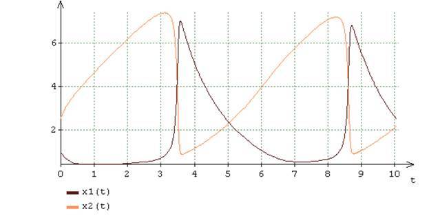t),r=1,2$ , , , $$$\lambda\_{n}, n=1,2$ , , «» $$. , , «», , , .

Fig.1. $$$(16)$ A = 2, B = 6 $$$(16)$ .

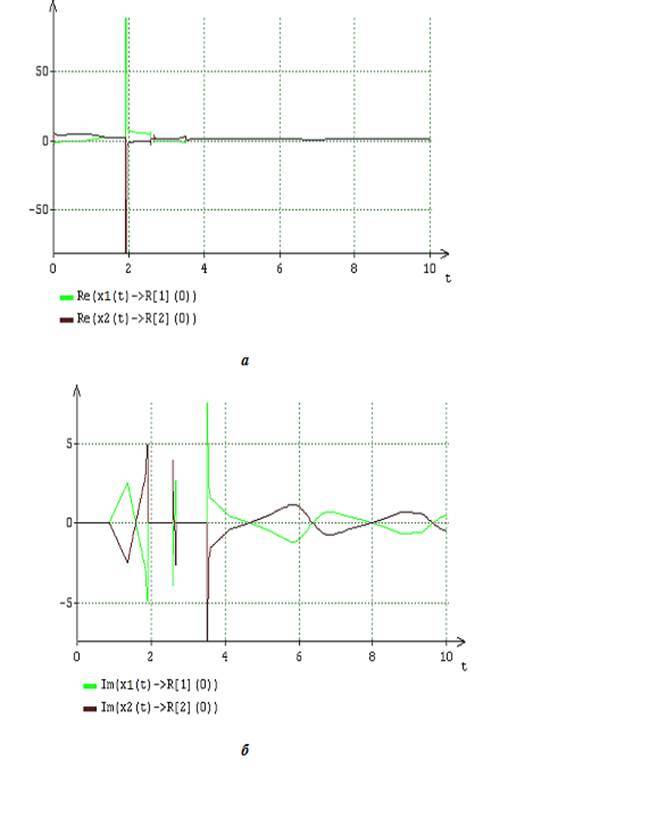
«» . 2-4. $$$(11)$ - $$$(13)$ , $$$N\_{m} =N=2$ and $$$l=1,2$ $$$x\_{l} (t)=x\_{l}^{+} (t)$ $$$(16)$ $$$\lambda\_{n}, n=1,2$ . , , .2 $$$\la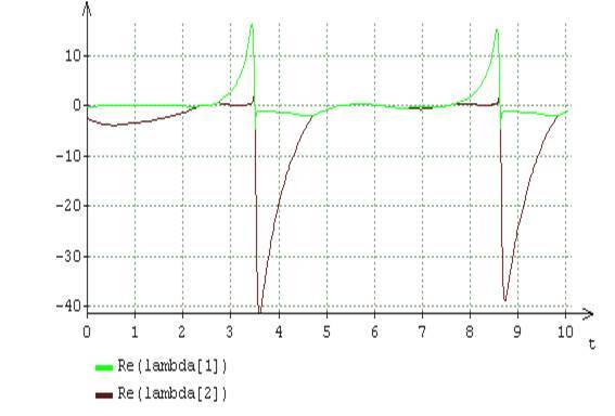mbda\_{n},n=1,2$ $$$(16)$ . , «», ,

()

()
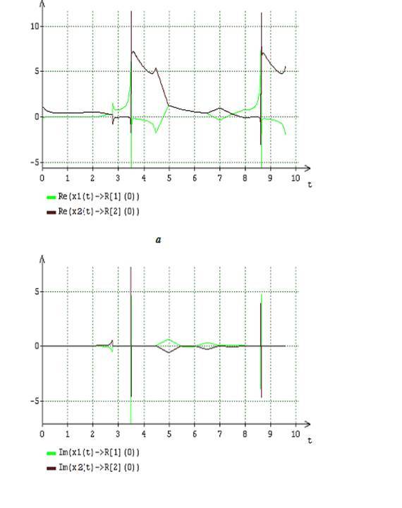
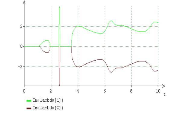
Fig.2. () () $$$\lambda\_{n}, n=1,2$ A= 2, B = 6

$$

$$\textbf{}$$

Fig.3. () () (13), $$${l=1,n}=1,2$ $$$x\_{1}(t)$ (16) A = 2, B = 6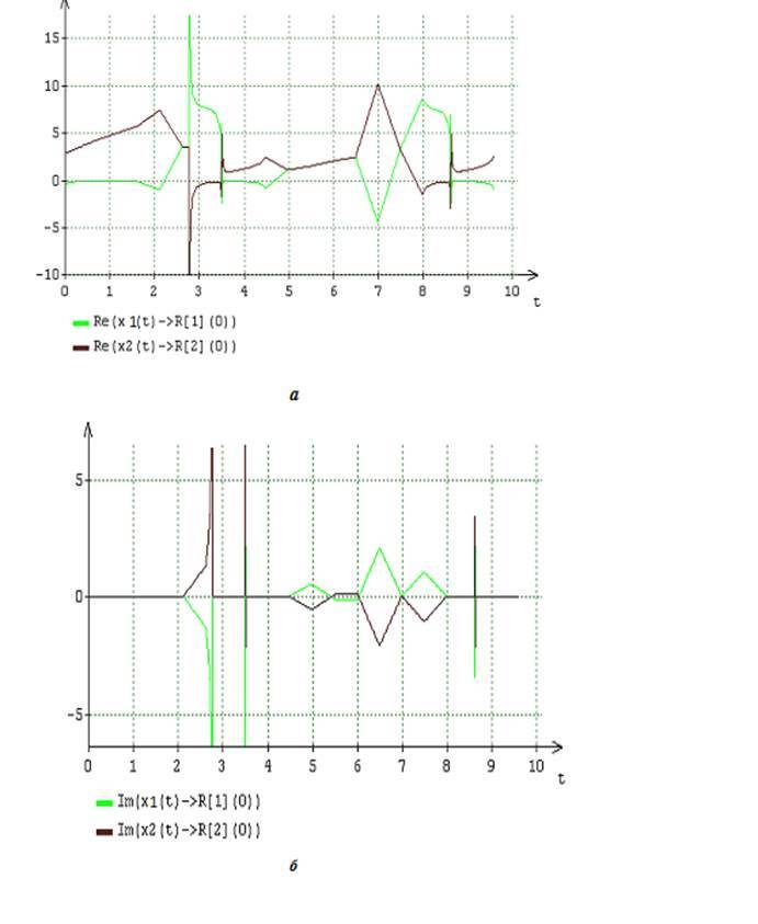

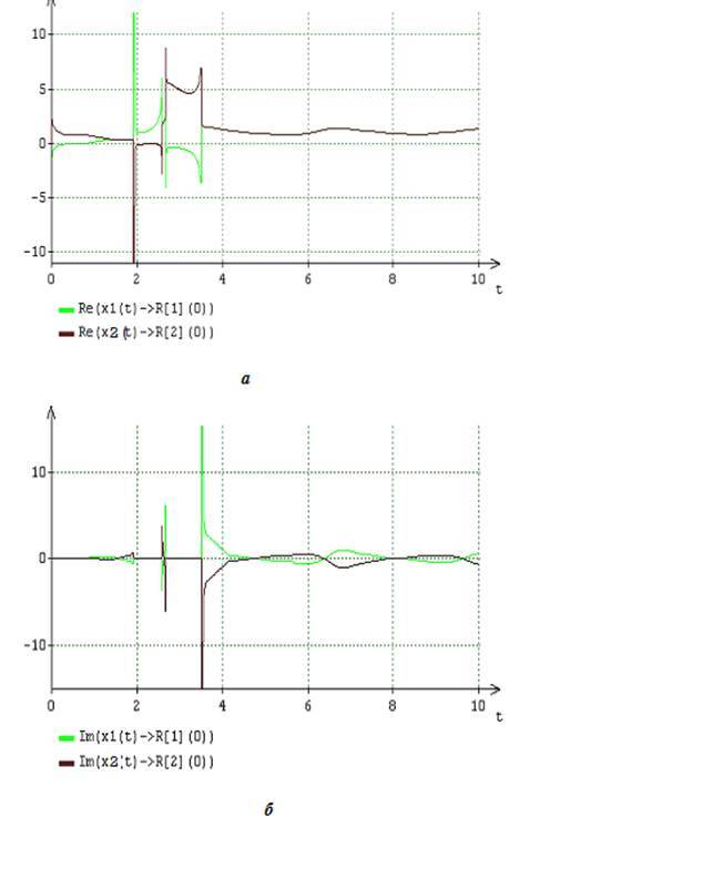
Fig.4. () () (13), $$$l=2, n=1,2$ $$$x\_2(t)$ (16) A = 2, B = 6

[0-10] $$$\lambda\_{n}, n=1,2$ , $$$\lambda\_{n}(t)$ . , $$$(16)$ . , .2, $$$\lambda\_{n}(t)$ , . , $$$(16)$ , . , , , , $$$\lambda\_{n}(t), n=1,2$ . $$$(16)$ : $$$=A^{2}+1$ .

$$$\lambda\_{n}, n=1,2$ , , $$$(9)$ , $$$(10)$ $$$(11)-(13)$ , $$$x\_{{\kern 1pt} l}^{\left[n\right]} \left(t\right)$ , $$$n=1,2, l=1,2$ $$$x\_{l} (t)$ $$$(16)$ . [0 -2,5] [4 -6,5], , , .1,3,4 , , $$$x\_{{\kern 1pt} l}^{\left[n\right]} \left(t\right)$ , $$$n=1,2, l=1,2$ $$$x\_{l} (t)$ , $$$(12)$ , $$$N=2,l=1,2$ , $$$x\_{l}^{+} (t\_{k} ;{\rm \; }I\_{l} )$ . $$$x\_{{\kern 1pt} l}^{\left[n\right]} \left(t\right)$ , $$$n=1,2, l=1,2$ $$$x\_{l} (t)$ , $$$x\_{l}^{+} (t\_{k} ;{\rm \; }I\_{l} )$ . , $$$(16)$ $$$x\_{l}^{+} (t\_{k} ;{\rm \; }I\_{l} )$ - .

[3 — 4] [7 — 8], , .1,3,4 , $$$(16)$ , , $$$x\_{{\kern 1pt} l}^{\left[n\right]} \left(t\right)$ , $$$n=1,2, l=1,2$ , , $$$\lambda\_n, n=1,2$ , . $$$x\_{{\kern 1pt} l}^{\left[n\right]} \left(t\right)$ , $$$n=1,2, l=1,2$ $$$x\_{l} (t)$ $$$\lambda\_n, n=1,2$ , .2 . $$$x\_{{\kern 1pt} l}^{\left[n\right]} \left(t\right)$ , $$$n=1,2, l=1,2$ $$$x\_{l} (t)$ , . -. , $$$x\_{1}(t)$ , .3 , $$$x\_{{\kern 1pt} l}^{\left[n\right]} \left(t\right)$ , $$$n=1,2, l=1,2$ , .4, , $$$x\_{{\kern 1pt} 2}^{[1]}(t)$ , $$$x\_{{\kern 1pt} 2}^{\left[2\right]} \left(t\right)$ . , $$$(16)$ , $$$x\_{{\kern 1pt} l}^{\left[n\right]} \left(t\right)$ , $$$n=1,2, l=1,2$ $$$x\_{l} (t), l=1,2$ .

$$$(16)$ , , , .5-8. , $$$(16)$$$$A = 2, B = 5.$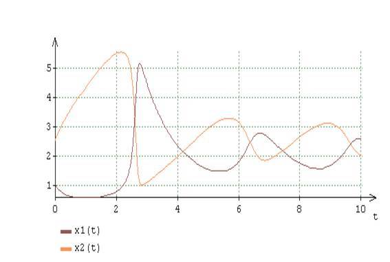

Fig.5. (16) A = 2, B = 5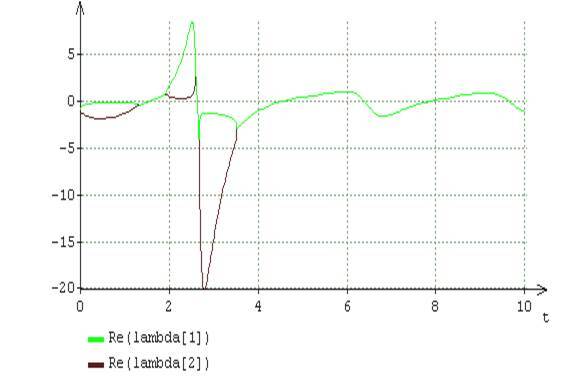

$$

$$\textbf{}$$

$$

$$\textbf{}$$

.6. () () $$$\lambda\_{n}, n=1,2$ (16) A = 2, B = 5

.7. () () (13) $$$N=2, l=1$ $$$x\_{1 }(t)$ (16) A = 2, B = 5

.8. () () (13) $$$N=2, l=2$ $$$x\_{2}(t)$ (16) A = 2, B = 5

, , $$$A = 2, B = 6.$

.5 $$$(16)$ at $$$A = 2, B = 5$ , $$$=A^{2}+1$ , $$$>(A^{2}+1)$ , :$$x_1(t)=;x_2(t)=$x\_{1}(t)=; x\_{2}(t)=\frac$ . , .6-8, $$$\lambda\_{n},n=1,2$ $$$(13)$ at $$$l=1,2$ and $$$n=1,2$ $$$x\_{{\kern 1pt} l}^{\left[n\right]} \left(t\right)$ $$$x\_{l} (t)$ .

.6 $$$\lambda\_n, n=1,2$ $$${A} = 2$ and $$$B = 5$ . .6 , $$${t}=3,5$ $$$\lambda\_n, n=1,2$ . .2 , , . , , $$$x\_{l} (t), l=1,2$ $$$(16)$ $$$(A=2, B=6)$ $$$(A=2, B=5)$ , , , $$$\lambda\_n, n=1,2$ , .

.5 , $$$(16)$ «». $$$(A=2, B=6)$ $$$t$ , $$$\lambda\_n, n=1,2$ , . $$$(16)$ , $$$A=2, B=5$ , - . , «» $$$(16)$ , , $$$\lambda\_n, n=1,2$ , .

$$$x\_{{\kern 1pt} l}^{\left[n\right]} \left(t\right)$ , $$$n=1,2, l=1,2$ $$$x\_{l} (t)$ $$$(16)$ , $$$\lambda\_n, n=1,2$ . , .3,4 .7,8 , , $$$(A=2, B=6)$ $$$(A=2, B=5)$ $$$x\_{{\kern 1pt} l}^{\left[n\right]} \left(t\right)$ , $$$n=1,2, l=1,2$ $$$x\_{l} (t)$ . , $$$x\_{{\kern 1pt} l}^{\left[n\right]} \left(t\right)$ , $$$n=1,2, l=1,2$ $$$x\_{l} (t), l=1,2$ . .7,8 . , , $$$x\_{l} (t), l=1,2$ $$$(16)$ $$$(A=2, B=6)$ $$( A = 2 , B = 5 ) , is the exclusion of any dominance among the components$(A=2, B=5)$$$$x\_{{\kern 1pt} l}^{\left[n\right]} \left(t\right)$ , $$n = 1 , 2 , l = 1 , 2 in the formation of dynamic indicators of the desired solutions$n=1,2, l=1,2$$$$x\_{l} (t)$ .

Bibliography

1. Danilov L.V., Matkhanov P.N., Filippov E.S. The theory of nonlinear electrical circuits. - L .: Energoatomizdat, 1990. - 256 p.
2. Haken G. Synergetic. The hierarchy of instabilities in self-organizing systems and devices. - M .: Mir, 1985. - 423 p.
3. Kronover R.M. Fractals and chaos in dynamic systems. Fundamentals of the theory. –M .: Postmarket, 2000. –352 p.
4. Heirer E., Nersett S., Vanner G. The solution of ordinary differential equations. Soft tasks / Trans. from English I.A. Kulchitskaya, S.S. Filippova (ed.) - M .: Mir, 1990. –512 p.
5. Zaslavsky G.M., Sagdeev R.Z., Usikov D.A., Chernikov A.A. Weak chaos and quasi-regular structures. - M .: Nauka, 1991.-240s.
6. Egorenkov DL, Fradkov A.L., Kharlamov V.Yu. Fundamentals of mathematical modeling with examples in MATLAB / Publishing house
   BSTU. - SPb., 1996. –192 p.
7. Andrievsky B.R. Analysis of systems in the state space. - SPb .: IPMash RAS, 1997. - 206 p.
8. Afanasyev V.N., Kolmanovsky V.B., Nosov V.R. Mathematical theory of designing control systems. –M .: Higher School., 1989. - 447 p.
9. Bychkov Yu.A., Scherbakov S.V. Analytical-numerical method for calculating dynamic systems. - Second edition, supplemented. St. Petersburg, Energoatomizdat, St. Petersburg Branch, 2002. - 368 p.
10. Bychkov Yu.A., Scherbakov S.V. Analytical and numerical calculation of deterministic nonlinear models of dynamic systems with lumped and distributed non-stationary parameters. Second edition, revised and updated. SPb .: Publishing house of Saint-Petersburg Electrotechnical University "LETI", 2014. - 388.